


Summary
In recent biomedical research, genome-wide association studies (GWAS) have demonstrated great success in investigating the genetic architecture of human diseases. For many complex diseases, multiple correlated traits have been collected. However, most of the existing GWAS are still limited because they analyze each trait separately without considering their correlations and suffer from a lack of sufficient information. Moreover, the high dimensionality of single nucleotide polymorphism (SNP) data still poses tremendous challenges to statistical methods, in both theoretical and practical aspects. In this article, we innovatively propose an integrative functional linear model for GWAS with multiple traits. This study is the first to approximate SNPs as functional objects in a joint model of multiple traits with penalization techniques. It effectively accommodates the high dimensionality of SNPs and correlations among multiple traits to facilitate information borrowing. Our extensive simulation studies demonstrate the satisfactory performance of the proposed method in the identification and estimation of disease-associated genetic variants, compared to four alternatives. The analysis of type 2 diabetes data leads to biologically meaningful findings with good prediction accuracy and selection stability.
1. Introduction
Genome-wide association studies (GWAS) in humans have been extensively conducted in biomedical research to identify a genotype–phenotype association. Recently, compared to a single trait, multiple correlated traits have been collected simultaneously in some GWAS, which usually share common biological mechanisms but which also have different implications. For example, in the analysis of type 2 diabetes in the Health Professionals Follow-up Study (HPFS) (Cornelis and others, 2010), both the body mass index (BMI) and weight are measured to determine the obesity level. Another example is the Northern Finland Birth Cohort 1966 (NFBC1966) (Järvelin and others, 2004), where four lipid traits, including total cholesterol, low-density lipoprotein, high-density lipoprotein, and triglycerides, were collected to study the risk factors of some diseases. However, most of the existing GWAS are still limited because they analyze each trait separately and do not effectively accommodate the correlations among multiple traits (Pan and others, 2014; Otowa and others, 2016). Compared to single-trait analysis, the joint analysis of multiple traits can investigate shared genetic variants with increased statistical power and identify pleiotropic loci in GWAS (Porter and O’eilly, 2017; Liang and others, 2018). The joint analysis of multiple responses has gained much success in low-dimensional biomedical studies. However, it is still very limited in high-dimensional studies. Recent joint analysis methods include Wu and others (2014) and Shi and others (2019).
To identify the disease-associated genetic variants, marker selection techniques are needed, among which the representative ones include multiple tests with multiple comparison adjustments (Pan and others, 2014) and regularized estimation with penalties (Shi and others, 2014). With the development of next-generation sequencing technologies, recent GWAS usually collect a large number of single nucleotide polymorphism (SNPs). However, the size of the subjects involved is still relatively small due to the sample, cost, and other constraints. As such, existing statistical methods often still have unsatisfactory results. For example, multiple tests with a large number of comparisons usually suffer from a substantial power loss. Regularization methods involve millions of parameters, leading to unstable estimation, inaccurate identification, and high computational complexity.
A simple example is illustrated in Figure 1. We simulate SNP data with a sample size |$n=150$| and dimension |$L=5000$| and generate one response with the true signals described by the solid grey line in Figure 1. A regression method with a SCAD penalty (Fan and Li, 2001) is conducted on discrete SNP data for a regularization estimation and marker selection, and the corresponding estimates are shown with blue points in Figure 1. The estimated values are observed as being much weaker, and they miss the majority of the true signals. Detections of disease-associated genetic variants when |$L$| is large are very challenging.
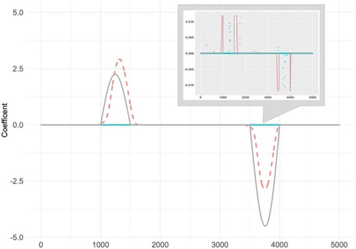
A simple example: true coefficient signals (grey solid line), estimated signals using the regression model with the smoothly clipped absolute deviation (SCAD) penalty (Fan and Li, 2001) (blue points), and estimated signals using the functional data analysis method fSCAD developed in Lin and others (2017) (orange dashed line). Upper right small plot: zoomed-in version with y-axis from |$-$|0.01 to 0.01.
To tackle these high dimensionality problems, recent GWAS have widely used functional data analysis. As large numbers of ordered genetic variants are located in very narrow regions, multiple genetic variants are treated as a continuum of sequence data rather than discrete variables (Fan and others, 2013), providing more satisfactory results compared to discrete SNP-based analysis. For example, a functional estimator with the fSCAD method, which was proposed by Lin and others (2017), is provided in Figure 1 and indicated by the orange dashed line, which effectively detects the true signals. Some novel functional data analysis methods have been developed for GWAS. For instance, Luo and others (2011) develop an association test based on a genome continuum model and functional principal components to detect the association of rare variants. Vsevolozhskaya and others (2014) propose a functional analysis of variance method to test the joint effect of gene variants, including both common and rare variants, with a qualitative trait. A few methodological developments for multiple traits are also conducted. Examples include Jadhav and others (2017), where a nonparametric functional U-statistic method is proposed to test the association between individuals’ sequencing data and multiple phenotypes. Lin and others (2017) introduce a quadratically regularized functional canonical correlation analysis with a likelihood ratio test for the association analysis of multiple traits. Despite considerable successes, the identified genetic variants have been shown to account for only a small fraction of disease heritability, and more effective GWAS analysis methods are very desirable (Porter and O’eilly, 2017; van Rheenen and others, 2019). Most existing studies, including the aforementioned, are based on hypothesis testing, and functional analysis for detecting disease-associated genetic variants still needs state of the art techniques.
Motivated by the tremendous challenges of GWAS in relation to high-dimensional SNPs and multiple correlated traits, and the demand for more effective genetic variant detection models, we propose a novel integrative method by jointly analyzing multiple traits with functional methods to approximate genetic variants and penalization techniques for smooth estimation and marker selection. Significantly advancing from existing single-trait analysis (Luo and others, 2011; Vsevolozhskaya and others, 2014; Lin and others, 2017), we jointly analyze multiple traits to improve statistical power and enhance our understanding of complex diseases, where traits’ correlations are effectively accounted for. Furthermore, significantly advancing from a discrete SNP-based analysis (Shi and others, 2014; Wu and others, 2014), we adopt functional data analysis and assume that high-dimensional genetic data follow a continuous process. It not only naturally accommodates correlations among adjacent SNPs but also avoids the unstable estimation of a large number of parameters. This is especially desirable with the rapidly increasing dimensions of SNP data but still limited sample size. In addition, unlike the testing strategy-based functional data analysis (Jadhav and others, 2017; Lin and others, 2017), the proposed method is based on penalization techniques, with a solid statistical foundation and the potential to be effectively realized. Overall, the proposed method provides a useful new venue for detecting disease-associated genetic variants in GWAS with multiple traits.
2. Methods
Consider |$n$| i.i.d subjects. For the |$i$|th subject, we denote |$\boldsymbol{y}_i=(y_ {i1}, \ldots, y_{iJ})$| as the vector of |$J$| traits and |$\boldsymbol{G}_{i} = (g_i(t_1), \dots, g_i(t_L))$| as the measurement vector of |$L$| SNPs which are located in a normalized region with ordered physical locations |$0 \le t_1 < t_2 < \cdots \le t_L = T=1$|. Here, |$g_i(t_l)\in \{0,1,2\}$| is the number of minor alleles for the |$i$|th subject and the |$l$|th SNP at |$t_l$|. In this study, high-dimensional SNP data are treated as a continuous sequence. We denote |$X_i(t)$| as the genetic variant function of the |$i$|th subject, which can be estimated based on the measurements |$g_i(t_1), \dots, g_i(t_L)$| of |$L$| discrete SNPs using some smooth estimation techniques. Specifically, consider the ordinary linear square smoother (Fan and others, 2013) with |$X_{i}(t)=\left(g_{i}\left(t_{1}\right), \ldots, g_{i}\left(t_{L}\right)\right) \boldsymbol{\Phi} \left[ \boldsymbol{\Phi} ^{\prime} \boldsymbol{\Phi} \right]^{-1} \phi(t),$| where |$\phi(t)=(\phi_1(t), \dots, \phi_{K}(t))'$| is the vector of basis functions and |$\boldsymbol{\Phi}$| is an |$L\times K$| matrix consisting of |$\phi_k(t_l), k=1,\ldots, K, l=1,\ldots, L$|.
2.1. Integrative functional linear model
Here, we introduce two modified variables |$\tilde{\boldsymbol{y}}_i=\boldsymbol{y}_i\boldsymbol{\Sigma}^{-1/2} $| and |$\tilde{\boldsymbol{\beta}}(t) = \boldsymbol{\beta}(t)\boldsymbol{\Sigma}^{-1/2} $|. In the first penalty term, |$\frac{M}{T} \int_{0}^{T} p_{\lambda_1}(|\tilde{\beta}_j(t)|) {\rm d} t\approx \sum\limits_{m=1}^{M} p_{\lambda_1}\left(\frac{\|\tilde{\beta}_{j,[m]}\|_{2}}{\sqrt{T / M}}\right)$| is the functional generalization of ordinary SCAD (fSCAD), where |$||\tilde{\beta}_{j,[m]}||_{2}=\sqrt{\int_{t_{m-1}}^{t_{m}} \tilde{\beta}_j^{2}(t) {\rm d} t}$|, |$p_{\lambda_1}(v)=\lambda_1 v I(0\leq v\leq \lambda_1)-\frac{v^2-2a\lambda_1 v+\lambda_1^2}{2(a-1)}I(\lambda_1< v< a\lambda_1)+\frac{(a+1)\lambda_1^2}{2}I(v\geq a\lambda_1)$| with |$I(\cdot)$| being an indicator function and |$a$| being 3.7 as suggested by Fan and Li (2001), and |$M$| is a large enough constant. In the second penalty term, we denote |$\mathcal{D}^{2}$| as the 2|${\rm nd}$|-order differential operator, and |$||f(t)||=\sqrt{\int_0^T f^2(t){\rm d}t}$| as the |$L_2$| norm of a function |$f(t)$|. There are three tuning parameters |$\lambda_1$|, |$\lambda_2$|, and |$\lambda_3$|. The proposed estimate is defined as the minimizer of (2.2). Since SNPs are closely located in continuous regions of chromosomes and those that are physically close are often likely to have similar biological functions or statistical effects, we select a region that is opposed to individual SNPs utilizing the natural property of functional data analysis. This region-based strategy has also been adopted in a few recent SNP studies (Guo and others, 2016; Wu and others, 2020). Specifically, the nonzero subregions of |$\beta_j(t)$| correspond to the important SNPs that are associated with the |$j$|th trait. In the objective function (2.2), the first term is a reparameterized form of the negative log-likelihood function |$\log |\boldsymbol{\Sigma}|+\frac{1}{n}\sum_{i=1}^{n}\Big(\boldsymbol{y}_ { i } - \int _ { 0 } ^ { T } X_ { i } ( t )\boldsymbol{\beta}( t ) {\rm d}t \Big) \boldsymbol{\Sigma}^{-1} \Big( \boldsymbol{y}_ { i } - \int _ { 0 } ^ { T } X _ { i } ( t )\boldsymbol{\beta} ( t ) {\rm d} t \Big) ^ { \prime }$|, where the correlations between multiple traits are effectively accommodated with the covariance matrix |$\boldsymbol{\Sigma}$|. If |$\boldsymbol{\Sigma}$| is an identity matrix, each trait is then analyzed independently. Reparameterization is conducted to make the objective function scale-invariant and easier to compute. For each of the coefficient functions, the fSCAD penalty is imposed for marker selection. It was first developed in Lin and others (2017) for locally sparse estimation under the functional linear regression model with a single response. The fSCAD penalty is the functional generalization of the SCAD penalty, which has been demonstrated to have better theoretical and numerical performance than some other penalties such as LASSO. For a sufficiently large number of consecutive subintervals, the overall magnitude, that is, the |$L_2$| norm, of |$\tilde{\beta} _ { j } ( t )$| over each subregion |$[t_{m-1}, t_{m}]$| can be shrunk to zero, leading to a locally sparse estimate. To control the smoothness of the locally sparse estimator, an additional smooth penalty is employed based on the 2nd-order differential of |$\tilde{\beta}_j(t)$|, which is a popular choice in functional data analysis. Significantly advancing from existing studies, the similarity of the coefficients between multiple traits is accommodated using the last penalty term, where some common genetic variants across multiple traits can be effectively identified. Three tuning parameters |$(\lambda_1, \lambda_2, \lambda_3)$| are involved in the objective function, which is not uncommon in recent biomedical studies (Chai and others, 2017). With the complexity of complex diseases, adopting increasing advanced statistical techniques and complex models has become a popular trend. They often include multiple parameters and have been suggested to still be computationally feasible. If we set |$\lambda_3$| to 0, the objective function goes back to the multiple-trait problem without considering the similarity among traits.
2.2. Computation
The proposed algorithm consists of two steps: the estimation of the genetic variant function |$X_i(t)$| with |$\boldsymbol{G}_{i}$| and the optimization of the objective function (2.2). The first step includes a simple calculation and does not demand any special algorithm. For the basis function, |$\phi_k(t_l)$|, both the B-spline basis and the Fourier basis are examined. We consider the simulation scenarios of Case I (details on the data settings are presented in the next section) and provide the summary results in Table S2 of the Supplementary material available at Biostatistics online. It is observed that different basis functions lead to different performance levels, and neither of them can perform consistently better than the other under all scenarios, which is similar to what was observed for other functional data analysis (Fan and others, 2013). In this study, we adopt the B-spline basis function, as it is also a popular choice in recent publications (Fan and others, 2013; Jadhav and others, 2017). To optimize the objective function (2.2), we update |$\boldsymbol{\Sigma}$| and |$\tilde{\boldsymbol{\beta}}(t)$| alternately. First, we adopt the B-spline basis method to approximate the coefficient function |$\tilde{\boldsymbol{\beta}}(t)$|, in accordance with the first step. We denote |$\boldsymbol{B}(t)=(B_{1}(t), \dots, $||$B_{(M+d)}(t) )$| as the B-spline basis vector with the order of the B-spline function being |$d+1$| and the number of knots being |$M+1$|. Then each coefficient function is expanded as |$\tilde{\beta}_j(t) = \sum_{k=1}^{M+d} B_{k}(t) b_{kj}$| with an unknown coefficient vector |$\boldsymbol{b}_j=(b_{1j},\ldots,b_{(M+d)j})'$| for |$j=1,2,\ldots, J$|.
To update |$\boldsymbol{\Sigma}$|, we use the ordinary maximum likelihood estimator |$\boldsymbol{\Sigma}=\frac{1}{n} \big(\boldsymbol{Y}-\boldsymbol{U} \boldsymbol{b}^*\big)'\big(\boldsymbol{Y}-\boldsymbol{U} \boldsymbol{b}^*\big)$|, where |$\boldsymbol{Y}=(\boldsymbol{y}'_ {1},\ldots,\boldsymbol{y}'_ {n})'$| and |$\boldsymbol{b}^*=(\boldsymbol{b}_1,\ldots,\boldsymbol{b}_J)\boldsymbol{\Sigma}^{1/2}$|. We adopt this estimator instead of optimizing the objective function (2.2), as it is computationally simpler and leads to satisfactory numerical results.
In summary, the proposed algorithm for optimizing (2.2) has these steps:
Step 1: Initialize |$s=0$|, |$\boldsymbol{\Sigma}^{(s)}=\frac{1}{n} \boldsymbol{Y}'\boldsymbol{Y}$|, |$\tilde{\boldsymbol{Y}}^{(s)}=\boldsymbol{Y}\left(\boldsymbol{\Sigma}^{(s)}\right)^{-1/2}$|, and |$\boldsymbol{b}^{(s)} = \left( {\breve{\boldsymbol{U}}}'\breve{{\boldsymbol{U}}} \right) ^ { - 1 }\breve{ {\boldsymbol{U}}}'\breve{\boldsymbol{Y}}^{(s)}$| with |$\breve{\boldsymbol{Y}}^{(s)}=\textrm{vec}\left(\tilde{\boldsymbol{Y}}^{(s)}\right)$|, where |$\boldsymbol{\Sigma}^{(s)}$|, |$\tilde{\boldsymbol{Y}}^{(s)}$|, |$\boldsymbol{b}^{(s)}$|, and |$\breve{\boldsymbol{Y}}^{(s)}$| denote the estimates of |$\boldsymbol{\Sigma}$|, |$\tilde{\boldsymbol{Y}}$|, |$\boldsymbol{b}$|, and |$\breve{\boldsymbol{Y}}$| at iteration |$s$|, respectively.
Step 2: Update |$s=s+1$|.
Compute |$\left(\boldsymbol{b}^*\right)^{(s)}=\left(\boldsymbol{b}_1^{(s-1)},\ldots,\boldsymbol{b}_J^{(s-1)}\right)\left(\boldsymbol{\Sigma}^{(s-1)}\right)^{1/2}$| and |$\boldsymbol{\Sigma}^{(s)}=\frac{1}{n} \big(\boldsymbol{Y}-\boldsymbol{U} \left(\boldsymbol{b}^*\right)^{(s)}\big)'\big(\boldsymbol{Y}-\boldsymbol{U} \left(\boldsymbol{b}^*\right)^{(s)}\big)$|;
Compute |$\breve{\boldsymbol{Y}}^{(s)}=\textrm{vec}\left(\tilde{\boldsymbol{Y}}^{(s)}\right)$| with |$\tilde{\boldsymbol{Y}}^{(s)}=\boldsymbol{Y}\left(\boldsymbol{\Sigma}^{(s)}\right)^{-1/2}$| and |$\boldsymbol{W}^{(s)}$| with |$\boldsymbol{b}^{(s-1)}$|;
Compute |$\boldsymbol{b}^{(s)}=\left(\breve{\boldsymbol{U}}'\breve{\boldsymbol{U}}+ 2n \boldsymbol { W } ^ { (s) } + 2n\lambda_2 (\boldsymbol{1}_{J\times J}\otimes\boldsymbol{V}) + 2n \lambda_3(\boldsymbol{A}\otimes\boldsymbol{Z}) \right) ^ { - 1 }\breve{\boldsymbol{U}}'\breve{\boldsymbol{Y}}^{(s)}$|.
Step 3: Repeat Step 2 until convergence. In our numerical study, convergence is achieved if |$\frac{||\boldsymbol{b}^{(s)}-\boldsymbol{b}^{(s-1)}||}{||\boldsymbol{b}^{(s)}||}<10^{-4}$|.
The convergence of the proposed algorithm is observed in all our numerical studies. Three tuning parameters, |$\lambda_1$|, |$\lambda_2$|, and |$\lambda_3$|, are selected using grid search and 10-fold cross-validation. There are two further parameters, including the knot number and the order, that are involved in the B-spline basis function. Our investigation suggests that with the smoothness penalty, the value of the knot number is not important, as long as it is large enough. We set the number of knots to 70 (=|$M+1$|), which has also been adopted in Lin and others (2017). For the order, we first examine four values, including 4, 5, 6, and 7, under the simulation scenarios of Case I. Summary results are provided in Tables S3–S5 of the Supplementary material available at Biostatistics online. It is observed that compared to order |$=4$| or |$7$|, models with order |$=5$| or 6 behave slightly better. Overall, the proposed method is not very sensitive to the choice of order when it is in a sensible range. Thus, to reduce computing complexity, we fix the order of the B-spline basis as 5 (=|$d+1$|) in our numerical studies.
The proposed algorithm is computationally feasible. With the functional data analysis framework, the number of parameters involved in the objective function is just |$(M+d)J$|, which is much lower than those with discrete SNP-based analysis. Specifically, under a standard laptop configuration, with fixed tuning parameters, the proposed analysis takes about 2 s for a simulated dataset with 150 subjects and 5000 SNP measurements. With extremely high efficiency, the grid search for three tuning parameters does not lead to a high computational cost. We have developed an R code that implements the proposed method, as well as an example with simulated data to illustrate its usage. The code and example are publicly available at https://github.com/rucliyang/IntegrativeFunc.
3. Simulation
We simulate SNP data with ordered physical locations. Specifically, (i) Each simulated dataset has |$n=150$|, |$L=5000$|, and |$J=2$|. (ii) A two-step method is adopted to simulate SNP data coded with |$(0,1,2)$| for genotypes (aa, Aa, AA). We first generate the genetic variant function |$X_i(t)=\sum_{j=1}^{\tilde{M}} a_{ij} B_j(t)$|, which is assumed to be the underlying continuous process of the discrete SNP data, with |$\tilde{M}=101$| B-spline basis functions |$B_1(t),\ldots,B_{\tilde{M}}(t)$| and the corresponding coefficients |$a_{ij}$|. We consider two settings for |$a_{ij}$| to represent different SNP patterns, where |$a_{ij}$|’s are generated from a normal distribution |$\mathcal{N}(0,1)$| and a uniform distribution |$\mathcal{U}(-2,2)$|, respectively. Following in the footsteps of previous studies (Liu and others, 2014; Wu and Ma, 2019; Santos and others, 2020), we conduct a trichotomization strategy to generate discrete SNP measurements. Specifically, consider a single locus with two alleles |$a$| and |$A$| having frequencies |$p_a=0.5$| and |$p_A=1-p_a=0.5$|, respectively. With the Hardy–Weinberg equilibrium assumption, the frequencies of genotypes |$(aa, Aa, AA)$| are set to |$(p_a^2, 2p_a p_A, p_A^2)=(0.25, 0.5, 0.25)$|. Thus, for |$l=1,\ldots,L$| and |$t\in [0,1]$|, we categorize the continuous values |$X_i(l/L)$| at its first and third quartiles to generate 3-level SNP measurements (0,1,2). (iii) For the coefficient function |$\beta_1(t)$|, we consider three settings for the lengths of signal regions: 20% (Case I), 10% (Case II), and 30% (Case III). (iv) For |$\beta_2(t)$|, we set three levels of similarity with |$\beta_1(t)$|. The first function |$\beta_{21}(t)$| has the same signal regions and shape as |$\beta_1(t)$|, but has a smaller magnitude of signals; the second one |$\beta_{22}(t)$| has the same signal regions and a similar magnitude of signals as |$\beta_1(t)$|, but a different shape; the third one |$\beta_{23}(t)$| has longer length of signal regions than |$\beta_1(t)$| and a different shape. A graphical presentation of |$\beta_1(t)$| and |$\beta_2(t)$| under Case I is illustrated in Figure 2. Figures of the other two cases and detailed equations of all cases are shown in Appendix A of the Supplementary material available at Biostatistics online. (v) Two correlated traits are generated based on (2.1), where the random error vector follows the multivariate normal distribution |$N(\boldsymbol{0},\boldsymbol{\Sigma})$|. We set two levels of correlations between two traits, that is,
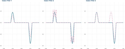
Simulation: true coefficient functions under scenario of Case I (20% signal region). Blue solid line: |$\beta_1(t)$|; Pink dashed line: |$\beta_2(t)$|. Left: |$\beta_1(t)$| and |$\beta_{21}(t)$|; Middle: |$\beta_1(t)$| and |$\beta_{22}(t)$|; Right: |$\beta_1(t)$| and |$\beta_{23}(t)$|.
In addition to the proposed method (M1), four alternatives are conducted. M2 analyzes the discrete SNP data directly and each trait independently using the penalized regression model with a spline-SCAD penalty developed by Guo and others (2016). The SCAD and spline penalty terms are adopted for sparse and smooth estimation, respectively, where the correlations among closely located SNPs are effectively accommodated. M3 is the same as M2 except for the absence of the spline penalty term. M4 is the functional data analysis method with fSCAD and smooth penalties developed in Lin and others (2017), where two traits are analyzed independently. M5 is the same as M4, except for the fact that the smooth penalty is not imposed, and the number of knots is selected using cross-validation. For two discrete SNP-based alternatives M2 and M3, to make all methods comparable, the coefficient functions are derived based on the estimated discrete coefficients. Comparing these alternatives can intuitively reveal the values of the proposed joint analysis of multiple traits and a functional data analysis strategy.
Four measures are used to evaluate model performance on the aspects of identification, estimation, and prediction, which are computed separately for each trait. First, the functional generalizations of true positive (TP) and false positive (FP) are employed to evaluate identification ability. We denote |$\eta_s(f(t))$| and |$\eta_0(f(t))$| as the lengths of the signal and zero regions of the function |$f(t)$|, respectively. We define TP|$ = \frac{\eta_s(\hat{\beta}(t)\beta(t))}{\eta_s(\beta(t))}$| and FP |$= \frac{\eta_s(\hat{\beta}(t)) -\eta_s(\hat{\beta}(t)\beta(t))}{\eta_0(\beta(t))}$|, where |$\hat{\beta}(t)$| and |$\beta(t)$| are the estimated and true coefficient functions. Second, the integrated squared error (ISE), defined as ISE |$=\int_0^T \big(\hat{\beta}(t) - \beta(t) \big)^2 {\rm d}t\big/\int_0^T \beta(t)^2 {\rm d}t$|, is used to examine the estimation property. Finally, an independent testing set with the same sample size is simulated for the prediction evaluation, and the predicted mean square error (PMSE) is adopted as the evaluation measure.
For each scenario, 100 replications are simulated. The summarized results, including the mean and standard deviation, under Case I of |$\beta_{1}$| paired with |$\beta_{21}, \beta_{22}$|, and |$\beta_{23}$| are shown in Tables 1, 2, and 3, respectively. The rest of the results are shown in Appendix B of the Supplementary material available at Biostatistics online. The proposed method is observed to have superior or competitive performance compared to the alternative methods across all scenarios. For example, in Table 1, consider the scenario under Case I with |$\mathcal{U}(-2,2)$|, correlation 0.6, and |$\beta_{21}(t)$|, where the two coefficient functions have identical signal regions, the same shape, but a different magnitude of signals. For both coefficient functions, the proposed method can identify the majority of signal regions with low FP. Specifically, the TP values of two functions are (0.980, 0.980) for M1, compared to (0.983, 0.516) for M2, (0.984, 0.512) for M3, (1.000, 0.986) for M4, and (0.976, 0.924) for M5, and the FP values are (0.317, 0.317) for M1, (0.800, 0.259) for M2, (0.814, 0.263) for M3, (0.730, 0.527) for M4, and (0.512, 0.297) for M5. The proposed method also has the lowest estimation errors. Under the above specific setting, the proposed method has the ISE values of (0.229, 0.273), compared to (0.736, 0.942) for M2, (0.722, 0.938) for M3, (0.377, 0.332) for M4, and (0.561, 0.491) for M5. To provide a more lucid demonstration, we show the true and estimated curves of coefficient functions under the scenario of Case I with |$\mathcal{N}(0,1)$|, correlation 0.9, and |$\beta_{23}(t)$| in Figure 3. The proposed M1 provides a much more accurate estimation. It also behaves better in prediction performance with the PMSE being (0.717, 0.725), compared to (0.916, 2.049) for M2, (0.911, 2.039) for M3, (0.750, 0.772) for M4, and (0.773, 0.760) for M5 under the scenario of Case I with |$\mathcal{U}(-2,2)$|, correlation 0.9, and |$\beta_{21}(t)$|. With the higher levels of correlation between two traits and similarity between two coefficient functions, the superiority of the proposed method become prominent. Cases II and III examine whether the proposed method has stable performance when the length of signal regions changes. Similar performance patterns are observed, where the proposed method performs better than alternatives by comprehensively considering all evaluation measures.
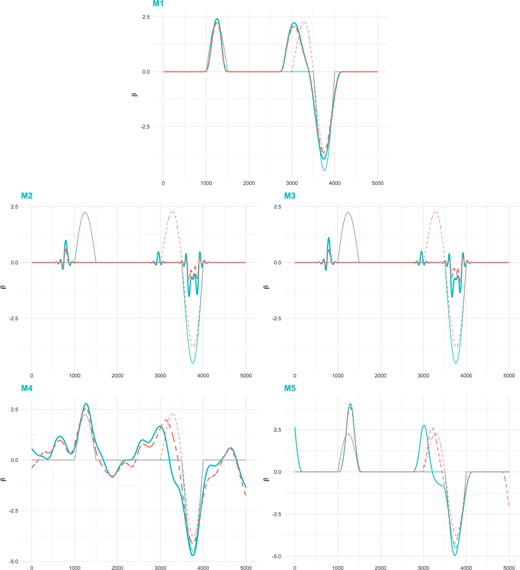
Simulation: true and estimated coefficient functions under scenario of Case I with |$\mathcal{N}(0,1)$|, correlation 0.9 and |$\beta_{23}(t)$|. Blue solid line (thin): |$\beta_1(t)$|; Blue solid line (thick): |$\hat{\beta}_1(t)$|; Orange dashed line (thin): |$\beta_{23}(t)$|; Orange dashed line (thick): |$\hat{\beta}_{23}(t)$|.
Simulation results under the scenarios of Case I with |$\beta_1(t)$| and |$\beta_{21}(t)$|. In each cell, mean (SD) based on 100 replicates.
| |$\beta_1(t)$| | |$\beta_{21}(t)$| | |||||||
|---|---|---|---|---|---|---|---|---|
| TP | FP | ISE | PMSE | TP | FP | ISE | PMSE | |
| |$a_{ij}\sim \mathcal{N}(0,1)$|, |${\rm cor}(y_1,y_2)=0.6$| | ||||||||
| M1 | 0.979 (0.099) | 0.305 (0.176) | 0.181 (0.099) | 0.711 (0.070) | 0.979 (0.099) | 0.305 (0.176) | 0.192 (0.105) | 0.713 (0.072) |
| M2 | 0.880 (0.257) | 0.634 (0.232) | 0.844 (0.115) | 0.947 (0.050) | 0.329 (0.246) | 0.160 (0.149) | 0.972 (0.034) | 2.197 (0.253) |
| M3 | 0.891 (0.230) | 0.654 (0.218) | 0.832 (0.111) | 0.943 (0.048) | 0.342 (0.246) | 0.169 (0.152) | 0.970 (0.036) | 2.186 (0.248) |
| M4 | 0.988 (0.071) | 0.699 (0.322) | 0.259 (0.110) | 0.726 (0.074) | 0.901 (0.239) | 0.483 (0.404) | 0.321 (0.203) | 0.760 (0.093) |
| M5 | 0.962 (0.101) | 0.440 (0.288) | 0.349 (0.144) | 0.754 (0.097) | 0.768 (0.345) | 0.252 (0.199) | 0.488 (0.289) | 0.808 (0.114) |
| |$a_{ij}\sim \mathcal{U}(-2,2)$|, |${\rm cor}(y_1,y_2)=0.6$| | ||||||||
| M1 | 0.980 (0.099) | 0.317 (0.189) | 0.229 (0.111) | 0.702 (0.082) | 0.980 (0.099) | 0.317 (0.189) | 0.273 (0.132) | 0.713 (0.083) |
| M2 | 0.983 (0.087) | 0.800 (0.139) | 0.736 (0.118) | 0.918 (0.050) | 0.516 (0.327) | 0.259 (0.199) | 0.942 (0.066) | 2.066 (0.310) |
| M3 | 0.984 (0.081) | 0.814 (0.131) | 0.722 (0.116) | 0.914 (0.052) | 0.512 (0.322) | 0.263 (0.197) | 0.938 (0.070) | 2.057 (0.310) |
| M4 | 1.000 (0.000) | 0.730 (0.294) | 0.377 (0.174) | 0.725 (0.080) | 0.986 (0.043) | 0.527 (0.375) | 0.332 (0.172) | 0.727 (0.073) |
| M5 | 0.976 (0.078) | 0.512 (0.320) | 0.561 (0.241) | 0.762 (0.100) | 0.924 (0.148) | 0.297 (0.231) | 0.491 (0.184) | 0.754 (0.094) |
| |$a_{ij}\sim \mathcal{N}(0,1)$|, |${\rm cor}(y_1,y_2)=0.9$| | ||||||||
| M1 | 0.988 (0.071) | 0.308 (0.195) | 0.212 (0.111) | 0.728 (0.065) | 0.988 (0.071) | 0.308 (0.195) | 0.221 (0.119) | 0.727 (0.072) |
| M2 | 0.879 (0.235) | 0.633 (0.245) | 0.850 (0.093) | 0.958 (0.038) | 0.325 (0.237) | 0.155 (0.128) | 0.969 (0.037) | 2.137 (0.155) |
| M3 | 0.894 (0.204) | 0.648 (0.232) | 0.837 (0.095) | 0.954 (0.038) | 0.335 (0.234) | 0.161 (0.123) | 0.968 (0.038) | 2.127 (0.155) |
| M4 | 0.994 (0.025) | 0.762 (0.279) | 0.302 (0.123) | 0.750 (0.080) | 0.920 (0.178) | 0.623 (0.369) | 0.346 (0.158) | 0.766 (0.091) |
| M5 | 0.952 (0.123) | 0.471 (0.285) | 0.418 (0.212) | 0.780 (0.086) | 0.902 (0.199) | 0.294 (0.196) | 0.405 (0.209) | 0.780 (0.092) |
| |$a_{ij}\sim \mathcal{U}(-2,2)$|, |${\rm cor}(y_1,y_2)=0.9$| | ||||||||
| M1 | 0.968 (0.124) | 0.281 (0.181) | 0.265 (0.192) | 0.717 (0.095) | 0.968 (0.124) | 0.281 (0.181) | 0.297 (0.206) | 0.725 (0.106) |
| M2 | 0.987 (0.073) | 0.800 (0.134) | 0.750 (0.121) | 0.916 (0.049) | 0.523 (0.281) | 0.284 (0.179) | 0.956 (0.042) | 2.049 (0.169) |
| M3 | 0.990 (0.071) | 0.813 (0.131) | 0.734 (0.125) | 0.911 (0.050) | 0.552 (0.297) | 0.311 (0.185) | 0.952 (0.045) | 2.039 (0.169) |
| M4 | 0.987 (0.070) | 0.752 (0.323) | 0.410 (0.203) | 0.750 (0.088) | 0.924 (0.249) | 0.613 (0.397) | 0.428 (0.241) | 0.772 (0.111) |
| M5 | 0.966 (0.102) | 0.487 (0.253) | 0.584 (0.282) | 0.773 (0.094) | 0.921 (0.151) | 0.249 (0.167) | 0.478 (0.188) | 0.760 (0.104) |
Simulation results under the scenarios of Case I with |$\beta_1(t)$| and |$\beta_{22}(t)$|. In each cell, mean (SD) based on 100 replicates.
| |$\beta_1(t)$| | |$\beta_{22}(t)$| | |||||||
|---|---|---|---|---|---|---|---|---|
| TP | FP | ISE | PMSE | TP | FP | ISE | PMSE | |
| |$a_{ij}\sim \mathcal{N}(0,1)$|, |${\rm cor}(y_1,y_2)=0.6$| | ||||||||
| M1 | 0.997 (0.018) | 0.360 (0.243) | 0.215 (0.095) | 0.713 (0.069) | 0.997 (0.018) | 0.360 (0.243) | 0.308 (0.067) | 0.735 (0.068) |
| M2 | 0.868 (0.255) | 0.630 (0.209) | 0.839 (0.094) | 0.956 (0.044) | 0.957 (0.130) | 0.783 (0.181) | 0.821 (0.092) | 0.711 (0.097) |
| M3 | 0.884 (0.249) | 0.651 (0.206) | 0.828 (0.094) | 0.953 (0.045) | 0.985 (0.058) | 0.807 (0.155) | 0.809 (0.097) | 0.708 (0.097) |
| M4 | 0.994 (0.023) | 0.552 (0.358) | 0.257 (0.131) | 0.723 (0.075) | 0.994 (0.025) | 0.654 (0.299) | 0.358 (0.116) | 0.749 (0.070) |
| M5 | 0.966 (0.142) | 0.397 (0.296) | 0.384 (0.211) | 0.748 (0.102) | 0.978 (0.072) | 0.502 (0.291) | 0.523 (0.173) | 0.796 (0.091) |
| |$a_{ij}\sim \mathcal{U}(-2,2)$|, |${\rm cor}(y_1,y_2)=0.6$| | ||||||||
| M1 | 0.989 (0.071) | 0.340 (0.187) | 0.271 (0.124) | 0.697 (0.067) | 0.989 (0.071) | 0.340 (0.187) | 0.369 (0.117) | 0.719 (0.057) |
| M2 | 0.967 (0.121) | 0.793 (0.161) | 0.762 (0.110) | 0.926 (0.050) | 0.989 (0.071) | 0.874 (0.122) | 0.757 (0.087) | 0.678 (0.085) |
| M3 | 0.970 (0.120) | 0.795 (0.156) | 0.747 (0.112) | 0.921 (0.051) | 0.990 (0.071) | 0.883 (0.105) | 0.739 (0.090) | 0.674 (0.085) |
| M4 | 0.958 (0.170) | 0.638 (0.366) | 0.356 (0.178) | 0.719 (0.092) | 0.992 (0.033) | 0.703 (0.294) | 0.468 (0.130) | 0.735 (0.072) |
| M5 | 0.961 (0.104) | 0.409 (0.263) | 0.479 (0.200) | 0.725 (0.093) | 0.989 (0.031) | 0.513 (0.246) | 0.620 (0.188) | 0.760 (0.074) |
| |$a_{ij}\sim \mathcal{N}(0,1)$|, |${\rm cor}(y_1,y_2)=0.9$| | ||||||||
| M1 | 0.968 (0.119) | 0.369 (0.211) | 0.269 (0.112) | 0.729 (0.081) | 0.968 (0.119) | 0.369 (0.211) | 0.380 (0.107) | 0.752 (0.081) |
| M2 | 0.870 (0.237) | 0.601 (0.208) | 0.846 (0.091) | 0.952 (0.036) | 0.968 (0.120) | 0.781 (0.166) | 0.838 (0.077) | 0.709 (0.078) |
| M3 | 0.871 (0.237) | 0.619 (0.202) | 0.835 (0.094) | 0.948 (0.038) | 0.968 (0.120) | 0.783 (0.165) | 0.828 (0.077) | 0.706 (0.078) |
| M4 | 0.978 (0.099) | 0.605 (0.357) | 0.275 (0.121) | 0.727 (0.070) | 0.995 (0.020) | 0.717 (0.314) | 0.397 (0.105) | 0.751 (0.073) |
| M5 | 0.942 (0.171) | 0.415 (0.307) | 0.424 (0.186) | 0.758 (0.093) | 0.980 (0.077) | 0.492 (0.313) | 0.532 (0.183) | 0.794 (0.096) |
| |$a_{ij}\sim \mathcal{U}(-2,2)$|, |${\rm cor}(y_1,y_2)=0.9$| | ||||||||
| M1 | 0.990 (0.071) | 0.308 (0.215) | 0.275 (0.135) | 0.718 (0.074) | 0.990 (0.071) | 0.308 (0.215) | 0.403 (0.117) | 0.733 (0.076) |
| M2 | 0.989 (0.071) | 0.781 (0.116) | 0.735 (0.123) | 0.920 (0.048) | 1.000 (0.000) | 0.904 (0.102) | 0.726 (0.108) | 0.673 (0.074) |
| M3 | 0.990 (0.071) | 0.787 (0.116) | 0.722 (0.124) | 0.916 (0.049) | 1.000 (0.000) | 0.906 (0.102) | 0.712 (0.117) | 0.670 (0.074) |
| M4 | 0.997 (0.018) | 0.633 (0.356) | 0.352 (0.175) | 0.729 (0.073) | 0.999 (0.007) | 0.703 (0.321) | 0.485 (0.175) | 0.741 (0.077) |
| M5 | 0.966 (0.077) | 0.314 (0.232) | 0.466 (0.211) | 0.741 (0.072) | 0.980 (0.042) | 0.412 (0.288) | 0.650 (0.250) | 0.784 (0.097) |
Simulation results under the scenarios of Case I with |$\beta_1(t)$| and |$\beta_{23}(t)$|. In each cell, mean (SD) based on 100 replicates.
| |$\beta_1(t)$| | |$\beta_{23}(t)$| | |||||||
|---|---|---|---|---|---|---|---|---|
| TP | FP | ISE | PMSE | TP | FP | ISE | PMSE | |
| |$a_{ij}\sim \mathcal{N}(0,1)$|, |${\rm cor}(y_1,y_2)=0.6$| | ||||||||
| M1 | 0.990 (0.071) | 0.349 (0.204) | 0.227 (0.123) | 0.730 (0.078) | 0.899 (0.123) | 0.296 (0.210) | 0.249 (0.135) | 0.735 (0.081) |
| M2 | 0.940 (0.193) | 0.690 (0.176) | 0.802 (0.098) | 0.941 (0.042) | 0.894 (0.176) | 0.568 (0.221) | 0.871 (0.076) | 1.005 (0.166) |
| M3 | 0.960 (0.137) | 0.698 (0.154) | 0.789 (0.097) | 0.936 (0.041) | 0.910 (0.158) | 0.593 (0.208) | 0.859 (0.074) | 1.000 (0.164) |
| M4 | 0.976 (0.108) | 0.591 (0.375) | 0.275 (0.158) | 0.750 (0.091) | 0.961 (0.095) | 0.594 (0.391) | 0.263 (0.134) | 0.739 (0.084) |
| M5 | 0.980 (0.032) | 0.398 (0.285) | 0.388 (0.196) | 0.771 (0.090) | 0.910 (0.149) | 0.397 (0.298) | 0.401 (0.240) | 0.774 (0.112) |
| |$a_{ij}\sim \mathcal{U}(-2,2)$|, |${\rm cor}(y_1,y_2)=0.6$| | ||||||||
| M1 | 0.997 (0.012) | 0.344 (0.165) | 0.245 (0.099) | 0.705 (0.069) | 0.930 (0.106) | 0.280 (0.171) | 0.252 (0.174) | 0.721 (0.080) |
| M2 | 0.986 (0.076) | 0.799 (0.158) | 0.737 (0.116) | 0.913 (0.045) | 0.924 (0.137) | 0.671 (0.216) | 0.789 (0.098) | 0.967 (0.157) |
| M3 | 0.990 (0.071) | 0.810 (0.142) | 0.724 (0.116) | 0.910 (0.046) | 0.925 (0.136) | 0.687 (0.231) | 0.775 (0.098) | 0.964 (0.157) |
| M4 | 0.989 (0.071) | 0.678 (0.352) | 0.337 (0.147) | 0.721 (0.073) | 0.961 (0.106) | 0.645 (0.389) | 0.292 (0.114) | 0.724 (0.086) |
| M5 | 0.973 (0.082) | 0.443 (0.306) | 0.507 (0.190) | 0.746 (0.085) | 0.910 (0.143) | 0.386 (0.316) | 0.443 (0.194) | 0.756 (0.093) |
| |$a_{ij}\sim \mathcal{N}(0,1)$|, |${\rm cor}(y_1,y_2)=0.9$| | ||||||||
| M1 | 0.949 (0.151) | 0.328 (0.185) | 0.256 (0.145) | 0.741 (0.076) | 0.880 (0.140) | 0.269 (0.202) | 0.271 (0.154) | 0.746 (0.084) |
| M2 | 0.888 (0.208) | 0.631 (0.215) | 0.877 (0.084) | 0.961 (0.035) | 0.783 (0.236) | 0.472 (0.224) | 0.901 (0.075) | 0.989 (0.093) |
| M3 | 0.886 (0.222) | 0.654 (0.217) | 0.866 (0.084) | 0.957 (0.036) | 0.788 (0.250) | 0.501 (0.237) | 0.891 (0.077) | 0.985 (0.095) |
| M4 | 0.982 (0.076) | 0.691 (0.329) | 0.287 (0.110) | 0.746 (0.087) | 0.979 (0.063) | 0.680 (0.382) | 0.246 (0.110) | 0.734 (0.078) |
| M5 | 0.954 (0.157) | 0.383 (0.235) | 0.376 (0.175) | 0.770 (0.097) | 0.917 (0.130) | 0.378 (0.280) | 0.332 (0.169) | 0.747 (0.093) |
| |$a_{ij}\sim \mathcal{U}(-2,2)$|, |${\rm cor}(y_1,y_2)=0.9$| | ||||||||
| M1 | 0.960 (0.137) | 0.414 (0.236) | 0.331 (0.172) | 0.728 (0.075) | 0.912 (0.134) | 0.357 (0.254) | 0.335 (0.188) | 0.735 (0.078) |
| M2 | 0.976 (0.103) | 0.791 (0.155) | 0.734 (0.111) | 0.916 (0.042) | 0.927 (0.132) | 0.703 (0.184) | 0.787 (0.095) | 0.974 (0.107) |
| M3 | 0.987 (0.073) | 0.797 (0.134) | 0.718 (0.109) | 0.911 (0.042) | 0.938 (0.145) | 0.719 (0.167) | 0.773 (0.094) | 0.969 (0.108) |
| M4 | 0.992 (0.035) | 0.722 (0.338) | 0.387 (0.138) | 0.730 (0.071) | 0.960 (0.098) | 0.701 (0.390) | 0.383 (0.160) | 0.738 (0.065) |
| M5 | 0.959 (0.102) | 0.449 (0.294) | 0.540 (0.211) | 0.757 (0.083) | 0.934 (0.120) | 0.430 (0.300) | 0.477 (0.176) | 0.747 (0.088) |
4. Data analysis
We analyze the type 2 diabetes dataset from the HPFS, which is collected by the GENEVA genotyping center of MIT and Harvard. Type 2 diabetes has been shown to affect almost 10% of the U.S. adult population and is thus an increasing public concern. Meanwhile, HPFS data have been successfully used in many clinical and epidemiological studies since it was first launched in 1986. It has contributed to many recent analyses (Yang and others, 2019; Liu and others, 2020) and provides valuable information. The data are downloaded from dbGaP with the accession number phs000091.v2.p1. In this study, the traits of interest are the BMI and weight, which are frequently used to describe the subject’s obesity level. They measure overlapped but different features of the subject’s obesity level and may share some common genetic information. SNPs on chromosome 4 are analyzed, wherein changes have been shown to have a variety of effects including delayed growth and development, intellectual disability, heart defects, and other medical problems. We first remove SNPs with MAF |$<0.05$| or a deviation from the Hardy–Weinberg equilibrium, and we then impute missing values via fastPHASE, to get 2558 subjects with 40 568 SNPs. As the number of disease-related genetic variants is not expected to be large, prescreening is conducted to improve stability. The p-values of each SNP through the marginal linear model is calculated, and the region of 10 000 consecutive SNPs with the smallest sum of p-values are selected for downstream analysis, where the ordered physical locations of SNPs are not changed.
Analysis is conducted using the proposed method and four alternatives. Estimated coefficient functions are shown in Figure 4, illustrating the identified null and signal regions of two functional genetic variant effects. Compared to the discrete SNP-based methods M2 and M3, three functional data analysis methods lead to much smoother and sparser estimation. With the joint analysis strategy, the proposed method can effectively detect some common genetic variants. Detailed information of the identified SNPs, including their locations and genes that the SNPs belong to or are the closest to, are provided in the Supplementary Excel File available at Biostatistics online.
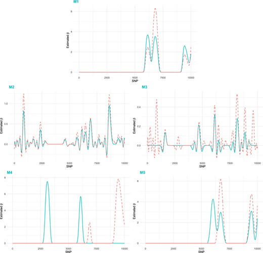
Data analysis: estimated coefficient functions. Blue solid line: |$\hat{\beta}_1(t)$|; Orange dashed line: |$\hat{\beta}_2(t)$|.
The proposed method identifies 116 distinct genes based on the estimated coefficient functions. The literature search suggests that most of the identified genes have important biological implications. For example, PPM1K not only increases the risk of developing type 2 diabetes but also regulates |$\beta$| cell insulin production and proliferation. Gene PDLIM5 has been suggested as a novel candidate gene, which probably plays a role in islets and in the context of diabetes. A high concentration of protein UNC5C has been indicated to be associated with end-stage kidney disease and structural lesions of diabetes. In a study identifying type 2 diabetes loci at regulatory hotspots in African Americans and Europeans, the regulation of the molecular functions of cis-genes PDHA2 has been detected as diabetes associated. A study of the hormonal activity of gene AIMP1 has shown that, in glucose homeostasis, AIMP1 plays a glucagon-like role and causes the increase of the blood glucose level. Gene HADH has been observed to have a significant expression in a meta-analysis of investigating diabetes-associated genes and pathways. Some other identified genes have been confirmed to play a critical role in obesity- or body weight-related studies. For example, the gene expression level of SPP1 has been shown to contribute to obesity-associated inflammation of peripheral blood mononuclear cells. Gene NAP1L5 has been found to be present in subjects with moderate obesity. Gene FAM13A has been demonstrated to be associated with adipose development and insulin sensitivity, and it has been identified as a candidate gene for fasting insulin. The genes GPRIN3, SNCA, MMRN1, and CCSER1 have also been found to be candidate genes in loci related to BMI and fasting serum insulin. The gene GRID2 has been demonstrated as a shared susceptibility gene in the neural synapse for substance use, obesity, stress, heart rate, and blood pressure traits. The over-expression of gene HPGDS has been observed in human adipose tissues, compared with lean subjects, suggesting that the inhibition of HPGDS may help control weight loss. A study has discovered a “phospho-switch” strategy that controls the stability of a tumor suppressor TET2 and can potentially help in cancer prevention and treatment. Gene PPA2 activation has been confirmed to be associated with a soluble form of tumor necrosis and is a weak inducer of apoptosis, which plays a significant role in obesity and type 2 diabetes.
In practical data analysis, it is difficult to objectively evaluate identification performance as the true signal regions are unknown. To provide partial support, we examine the prediction accuracy and selection stability, which are commonly adopted in existing studies. A resampling is conducted. The training data with 2/3 of all subjects is used to build a model and estimate parameters, and testing data with 1/3 of all subjects is used to evaluate the prediction. The average values of PMSE over 100 resamplings are (0.128, 0.128), (0.727, 0.669), (0.936, 0.849), (0.130, 0.129), and (0.129, 0.129) for M1, M2, M3, M4, and M5, respectively. The proposed method has competitive prediction accuracy compared to M4 and M5, and a much better prediction performance than M2 and M3. For the evaluation of selection stability, we adopt the functional generalization of the Jaccard coefficient (FJC), defined as the ratio of the length of the signal region identified from both original and resampling data to that identified from the original data. It takes values between 0 and 1, with a larger value indicating better selection stability. The proposed method has the average FJC value of (0.774, 0.774) for two traits, compared to (0.960, 0.991), (0.590, 0.748), (0.652, 0.748), and (0.798, 0.717) for M2, M3, M4, and M5, respectively. Satisfactory selection stability of the proposed method is observed, where M2 identifies a much denser signal region, resulting in a larger FJC value. The favorable prediction and stability performance provides support to the validity of the proposed analysis.
5. Discussion
With the burgeoning development of next-generation sequence technologies, millions of SNPs are usually collected in recent GWAS, and the high dimensionality poses immense challenges to statistical analysis. Another challenge comes from the need to accommodate the correlations among multiple traits. In this study, we have developed a new integrative method that jointly analyzes multiple traits and effectively accounts for the similarity between more than one trait to facilitate information borrowing. Functional data analysis has been adopted to exploit the naturally ordered physical locations of SNPs and accommodate the high dimension problems. We acknowledge that the values of SNP data are highly discrete, which may not be very common in traditional functional data estimation. However, functional data analysis of discrete SNP data is becoming a new trend in GWAS, where the effectiveness has been well established (Fan and others, 2013; Jadhav and others, 2017; Chiu and others, 2019). Extensive simulation studies with various patterns of discrete SNP data in our study have also provided strong support for the validity of the functional data analysis. Three penalty terms have been imposed for sparse, smooth, and similarity estimation, with an intuitive formulation and lower computational cost. Our numerical studies have revealed that consideration of the unknown correlation between two traits is necessary and can help improve the model performance of identifying, estimating, and predicting common genetic variants. The analysis of type 2 diabetes data has shown that the proposed method can select biologically meaningful genetic markers with satisfactory prediction accuracy and selection stability, providing suggestions for further clinical or epidemiological research.
Nonetheless, this study suffers from some limitations, which can be addressed by future research. This study has considered multiple continuous traits. It can be of interest to extend the proposed joint functional linear model to other data types, such as categorical and count traits. For example, the latent continuous variable-based strategy developed in Gueorguieva and Agresti (2001) can be potentially coupled with the proposed framework to accommodate both continuous and binary traits. We have mostly focused on the methodological development and implementation of the proposed method. The estimation and selection consistency of the locally sparse estimator for functional linear regression with a single trait has been rigorously established in Lin and others (2017). It is thus reasonable to conjecture that the proposed joint analysis may also have good statistical properties; we leave the detailed investigation to further research. The proposed method has adopted functional data analysis to naturally accommodate the adjacency structure of SNPs, where the distance of adjacency is not accounted for. It is sensible since many SNPs are densely located in a narrow region of the chromosome. The proposed method can be potentially extended to incorporate the distance of adjacency, if necessary, which may warrant a separate investigation. In the data analysis, we have identified some disease-associated genes with supportive clinical evidence. Others still need professional biological and functional examinations.
Supplementary material
Supplementary material is available at http://biostatistics.oxfordjournals.org.
Funding
The National Institutes of Health (CA204120, CA241699, CA216017); National Science Foundation (1916251); Yale Cancer Center Pilot Award; Bureau of Statistics of China (2018LD02); “Chenguang Program” supported by Shanghai Education Development Foundation and Shanghai Municipal Education Commission (18CG42); Program for Innovative Research Team of Shanghai University of Finance and Economics; Shanghai Pujiang Program (19PJ1403600); National Natural Science Foundation of China (12071273, 71771211); and Fundamental Research Funds for the Central Universities (2016110061, 2018110443).
Acknowledgments
We thank the editor and reviewers for their careful review and insightful comments, which have led to a significant improvement of this article.
Conflict of Interest: None declared.
