


Summary
We develop a scalable and highly efficient algorithm to fit a Cox proportional hazard model by maximizing the |$L^1$|-regularized (Lasso) partial likelihood function, based on the Batch Screening Iterative Lasso (BASIL) method developed in Qian and others (2019). Our algorithm is particularly suitable for large-scale and high-dimensional data that do not fit in the memory. The output of our algorithm is the full Lasso path, the parameter estimates at all predefined regularization parameters, as well as their validation accuracy measured using the concordance index (C-index) or the validation deviance. To demonstrate the effectiveness of our algorithm, we analyze a large genotype-survival time dataset across 306 disease outcomes from the UK Biobank (Sudlow and others, 2015). We provide a publicly available implementation of the proposed approach for genetics data on top of the PLINK2 package and name it snpnet-Cox.
1. Introduction
Survival analysis involves predicting time-to-event, such as survival time of a patient, from a set of features of the subject, as well as identifying features that are most relevant to time-to-event. Cox proportional hazard model (Cox, 1972) provides a flexible mathematical framework to describe the relationship between the survival time and the features, allowing a time-dependent baseline hazard. Survival analysis faces computational and statistical challenges when the predictors are ultrahigh-dimensional (when feature dimension is greater than the number of observations) and large scale (when the data matrix does not fit in the memory). Based on the Batch Screening Iterative Lasso (BASIL), we develop an algorithm to fit a Cox proportional hazard model by maximizing the Lasso partial likelihood function. We apply the method to 306 time-to-event disease outcomes from UK Biobank combined with genetic data. We generate improved predictive models with sparse solutions using genetic data with the number of variables selected ranging from a single active variable in the set and others with almost 2000 active variables. We note that our algorithm can be easily adapted to other applications with arbitrarily large dataset, provided that the Lasso solution is sufficiently sparse.
1.1. Cox proportional hazard model
Given a numerical predictor |$X \in \mathbb{R}^d$|, Cox model assumes that there exists a baseline hazard function |$h_0: \mathbb{R}^+ \mapsto \mathbb{R}^+$| and a parameter vector |$\beta \in \mathbb{R}^d$| such that the hazard function for survival time has the form:
Intuitively the hazard function at time |$t$| measures the relative risk of death around time |$t$|, given that the patient survives up to time |$t$|. Under Cox proportional hazard model, the hazard ratio between two subject with covariates |$X$| and |$X'$| can be written as:
When |$X$| is an indicator for a treatment, the hazard ratio can be interpreted as the risk of event occurring in the treatment group, compared to the risk in the control group, and the regression coefficient |$\beta$| is the log-hazard ratio.
To describe the distribution of the survival time, we can equivalently use its cumulative distribution function:
In practice, it is often the case that the survival time is right-censored. That is the event has not yet happened at the time the data was collected. Therefore for the |$i$|th individual, we observe a tuple |$(X_i, O_i, T_i)$|, where |$X_i \in \mathbb{R}^d$| is the predictors, |$O_i \in\{0, 1\}$| is the event indicator. If |$O_i = 1$|, then |$T_i$| is the actual survival time of the |$i$|th individual. If |$O_i = 0$|, then we only know that the true survival time of the |$i$|th individual is longer than |$T_i$|. Throughout this article, we will assume that the censoring is non-informative, meaning that the time of censoring is independent of the (possibly unobserved) event time conditional on |$X_i$|.
One advantage of the Cox model is that, while being a semi-parametric model (the baseline function is non-parametric), we could still estimate the parameter |$\beta$| without estimating the baseline function. This can be achieved by choosing |$\hat{\beta}$| that maximizes the log-partial likelihood function:
We use the C-index to evaluate a fitted |$\hat{\beta}$|:
The C-index is the proportion of comparable pairs for which the model |$\hat{\beta}$| predicts the correct order of the events. Each tie in the prediction is considered half of a correct prediction. For a more complete description of C-index, see Harrell and others (1982) and Li and Tibshirani (2019).
1.2. Computational challenges in large-scale and high-dimensional survival analysis
In today’s applications, it is common to have dataset with millions of observations and variables. For example, the UK Biobank dataset (Sudlow and others, 2015) contains millions of genetic variants for over 500 000 individuals. Loading this data matrix to R takes around |$2.4$| TB of memory, which exceeds the size of a typical machine’s RAM. While memory-mapping techniques allow users to perform computation on data outside of RAM (out-of-core computation) relatively easily (Kane and others, 2013), popular optimization algorithms require repeatedly computing matrix-vector multiplications involving the entire data matrix, resulting in slow overall speed.
The Lasso (Tibshirani, 1996) is an effective tool for high-dimensional variable selection and prediction. R packages such as glmnet (Friedman and others, 2010), penalized (Goeman, 2010), coxpath (Park and Hastie, 2007), and glcoxph (Sohn and others, 2009) solve Lasso Cox regression problem using various strategies. However, all of these packages require loading the entire data matrix to the memory, which is infeasible for Biobank-scale data. To the best of the authors’ knowledge, our method is the first to solve |$L^1$| regularized Cox regression with larger-than-memory data. On the other hand, most optimization strategies used in these packages can also be incorporated in the fitting step of our algorithm. In particular, snpnet-Cox uses cyclical coordinate descent implemented in glmnet.
Even if these packages do support out-of-core computation, using them directly would be computationally inefficient. To be more concrete, in one of our simulation studies on the UK Biobank data, the training data take about 2 TB. With the highly optimized out-of-core matrix-vector multiplication function PLINK2 provides, we are able to run one single such operation in about 2–3 min. Without variable screening, cyclic coordinate descent (or proximal gradient descent) would require from a few to tens or even hundreds of such matrix-vector multiplications for one |$\lambda$|. Our algorithm exploits the sparsity structure in the problem to reduce the frequency of this operation to mostly once or twice for several |$\lambda$|s. Most of these expensive, out-of-core matrix-vector multiplications are replaced with fast, in-memory ones that work on much smaller subsets of the data.
2. Methods
2.1. Preliminaries
We first introduce the following notations:
Let |$n, d$| be the number of observations and the number of features, respectively. Let |$\boldsymbol{X} \in \mathbb{R}^{n \times d}$| be the matrix of predictors. To simplify notation, we use |$n, d, \boldsymbol{X}$| for all of train, test, and validation set. Whether |$\boldsymbol{X}$| comes from train, test, or validation data can be inferred from the context.
Let |$X_i \in \mathbb{R}^d$| be the |$i$|th row of |$\boldsymbol{X}$|.
Let |$x_j \in \mathbb{R}^n$| be the |$j$|th column of |$\boldsymbol{X}$|.
- Denote the log-partial likelihood function as |$f(\beta)$|. That is(2.6)$$\begin{equation} f(\beta) = \sum_{i:O_i = 1} \beta^T X_i -\log \left(\sum_{j:T_j \ge T_i} \exp(\beta^T X_j)\right)\!.\end{equation}$$
Denote the set |$\{1,2,\ldots, n\} = [n]$|.
We focus on survival analysis in the high-dimensional regime, where the number of predictors is greater than the number of observations (|$d >n$|), although same procedure can easily be applied to low-dimensional cases. We use Lasso to perform variable selection and estimation at the same time. In particular, we optimize the |$L^1$|-regularized log-partial likelihood:
where the |$\|\beta\|_1 = \sum_{j=1}^d |\beta_j|$|. More generally, we allow each parameter or each observation to have a different weight in the objective function, the right-hand side of (2.7). In particular, given a vector of penalty factors |$w^p \in \mathbb{R}^d_+$|, and observation weight |$w^o \in \mathbb{R}^n_+$|, we define the general objective function to be
This can be particularly useful if we are considering genetic variants that we would like to up-weight during variable selection, e.g., coding variants in a region of perfect linkage disequilibrium. To simplify the notation, we describe our algorithm assuming that the parameters and the observations are unweighted.
2.2. Hyperparameter selection
To find the optimal hyperparameter |$\lambda$|, we start with a sequence of |$L$| candidate regularization parameters |$\lambda_1 > \lambda_2 > \cdots, \lambda_L > 0$| and compute the corresponding parameter estimate as well as the validation metric. The optimal regularization parameter is then selected to be |$\lambda_l$| that maximizes the validation metric and |$\hat{\beta}$| is set to be |$\hat{\beta}(\lambda_l)$|. The sequence of regularization parameters can be chosen by setting |$\lambda_1$| to be sufficiently large such that the optimal |$\hat{\beta}(\lambda_1)$| is just zero, and find |$L=100$| equally spaced |$\lambda$|s in log-scale.
Applying this procedure naively requires solving |$L$| optimization problems, each reading the entire predictor matrix |$\boldsymbol{X}$|. To effectively reduce the number of computations involving the entire data matrix, we exploit the sparsity of the Lasso solution. The key components of our algorithm that significantly speed up the computation are the following observations adapted from Qian and others (2019).
2.3. Batching screening procedure
The Karush–Kuhn–Tucker (KKT) condition of (2.7) indicates that the optimal |$\hat{\beta}(\lambda)$| must satisfy:
When |$\lambda$| is sufficiently large, |$\hat{\beta}(\lambda)$| is sparse, so our strategy is to solve the optimization problem (2.7) using only a small subset of features, assuming all the others have coefficient zero. Then, we verify that the solution satisfies the KKT condition (2.9). We iteratively apply this strategy for |$\lambda = \lambda_1,\ldots, \lambda_L$| to obtain the entire Lasso path. To determine which predictors to include in the model, we adopt the screening rules used in BASIL, which is inspired by the strong rules proposed in Tibshirani and others (2012). In Cox model, the strong rules assumes |$\hat{\beta}_j(\lambda_k) = 0$| (discard the |$j$|th predictor when fitting) if
By convention we set |$\lambda_0 = \infty$|. Although it is possible for strong rules to fail, it rarely happens when |$d > n$|.
Before we describe the full algorithm, first we write the gradient of the log-partial likelihood into a simple form. Notice that the gradient of the log-partial likelihood function can be written as:
Let |$r = r({\rm data},\beta) \in \mathbb{R}^n$| be defined as
Then by direct computation one can show that
Here, |$r$| is the martingale residual when the baseline survival function comes from a Breslow estimator (Barlow and Prentice, 1988; Breslow, 1974), and it can be computed using only variables currently in the model. However, based on its definition computing |$r$| requires summing over the risk set for each |$i$| (the denominator in the second term), which in total takes |$\mathcal{O}(n^2)$|. Our solution is to first sort the individuals based on |$T_i$|, so that |$T_1\le \cdots \le T_n$|. Then |$\sum_{k:T_k \ge T_j} \exp(\beta^T X_k) = \sum_{k:k \ge j} \exp(\beta^T X_k)$| can be obtained for all |$k \in [n]$| in |$\mathcal{O}(n)$|. The only expensive part then is the matrix multiplication above, which involves the large data matrix |$\boldsymbol{X}$|. Our full algorithm follows the same structure as in BASIL (Qian and others, 2019), where at each iteration of our algorithm we look for Lasso solution for multiple consecutive |$\lambda$|s in the Lasso path so that large dataset is not read in too frequently. Suppose |$\hat{\beta}(\lambda_0), \ldots, \hat{\beta}(\lambda_l)$| have been computed in the first |$k-1$| iterations, and the KKT condition for these solution has been verified. The |$k$|th iteration has the following parts:
(Screening) In the last iteration, we obtain |$r^{(k-1)}$| defined as the right-hand side of (2.12), which we will use to compute the full gradient through |$ \nabla_\beta f(\hat{\beta}(\lambda_l))= r^T\boldsymbol{X}$|. We include two types of variables in the fitting step of this iteration:
The set of variables |$j$| with |$\hat{\beta}_j(\lambda) \neq 0$| for some |$\lambda \ge \lambda_l$|. We call this set ever-active set at iteration |$k-1$|, denoted |$\mathcal{A}^{(k-1)} \subseteq [d]$|.
Top |$M$| variables with the largest partial derivative magnitude |$|\partial_{\beta_j}f(\hat{\beta}(\lambda_l))|$|, that are also not ever active.
The union of these two type of variables is denoted |$\mathcal{S}^{(k)} \subseteq [d]$|, and we will use this set of variables for the fitting step.
(Fitting) In this step we solve the problem (2.7) using the variables |$\mathcal{S}^{(k)}$|, for the next few (default |$5$|) |$\lambda$| values starting at |$\lambda_{l+1}$|. The set of |$\lambda$|s used in this iteration is denoted |$\Lambda^{(k)}$|. The solutions are obtained through coordinate descent, with iterates initialized from the most recent Lasso solution (warm start). The corresponding coefficients of the variables not in |$\mathcal{S}^{(k)}$| are set to |$0$|.
(Checking) In this step, we verify that the solutions obtained in the fitting step assuming |$\beta_j = 0$| for |$j \not\in \mathcal{S}^{(k)}$| is indeed valid. To do this, for each |$\lambda$| in this iteration, we obtain the martingale residual |$r$| as in (2.12), compute the gradient |$\nabla_\beta f(\hat{\beta}(\lambda)) = r^T\boldsymbol{X}$|, and verify the KKT condition (2.9). If |$\hat{\beta}(\lambda)$| satisfies the KKT condition, then it is a valid solution. Otherwise, we go back to the screening step and continue with the largest |$\lambda \in \{\lambda_1,\ldots,\lambda_L\}$| for which the KKT condition fails.
(Early Stopping) When the regularization parameter |$\lambda$| becomes small, the model tends to overfit and the solution we obtain becomes unstable. We keep a separate validation set to determine the optimal hyperparameter. For |$\lambda \in \Lambda^{(k)}$|, if |$\hat{\beta}(\lambda)$| satisfies the KKT condition, we evaluate its validation C-index. Once the validation C-index starts to decrease, we stop computing solution for smaller |$\lambda$| values. A naive implementation of C-index requires comparing |$\mathcal{O}(n^2)$| pairs of individuals in the study, which is not scalable. In the next section, we describe an |$\mathcal{O}(n\log n)$| C-index algorithm.
We emphasize that, in each iteration, only one matrix–matrix multiplication using the entire data set |$\boldsymbol{X}$| is needed (except the first iteration where |$2$| are needed). Algorithm 1 summarizes this procedure. The early stopping step is omitted to save some space.
BASIL for Cox model
2.4. Fast C-index computation
Several frequently used C-index computational algorithms, including the first algorithm we tried, have time complexity |$\mathcal{O}(n^2)$|. As population-scale cohorts, like UK Biobank, Million Veterans Program, and FinnGen, aggregate time-to-event data for survival analysis it is increasingly important to consider the computational costs of statistics like C-index to build and evaluate predictive models. The time-to-event data for survival analysis include age of disease onset, progression from disease diagnosis to another more severe outcome, like surgery or death. Here, we present an implementation with |$\mathcal{O}(n\log{}n)$| time complexity (and |$\mathcal{O}(n)$| space complexity) that can introduce over 10 000|$\times$| speedup for biobank-scale data relative to several R packages, and over 10|$\times$| speedup compared to existing |$\mathcal{O}(n\log n)$| time complexity (and |$\mathcal{O}(n + n\log n)$| space complexity) algorithm implemented in the survival analysis package by Therneau and Lumley (2014).
We first assume there are no tied predictions or events. We evaluate the C-index of the estimator |$\hat{\beta}$| on the data |$\{O_i, T_i, X_i\}_{i=1}^n$| through the following steps:
- First relabel the data in increasing |$T_i$|. This takes |$\mathcal{O}(n\log n)$|. After relabeling, we have$$\begin{equation*} T_1 < T_2 < \cdots < T_n.\end{equation*}$$Define$$\begin{equation*} R_i := |\{j \in [n]: T_j > T_i\}| = n - i \quad \text{for } i \in [n].\end{equation*}$$
|$R_i$| is the size of the risk set immediately after |$T_i$|. Clearly, computing all |$R_i$| takes |$\mathcal{O}(n)$|.
- Define$$\begin{equation*} u_i := |\{j: \hat{\beta}^TX_j \le \hat{\beta}^TX_i\}| \quad \text{for } i \in [n].\end{equation*}$$
That is, |$u_i$| is the number of individuals that |$\hat{\beta}$| predicts to have lower or equal risk of the event than |$i$|. We have |$u_i \in [n]$| for all |$i$|, and |$u_i > u_j$| is equivalent to |$\hat{\beta}^TX_i > \hat{\beta}^TX_j$|. The |$u_i$|’s can be computed in linear time by first sorting |$\boldsymbol{X}\hat{\beta}$| (here we assume |$\boldsymbol{X}\hat{\beta}$| has already been computed and given as an input to the C-index function). The total time complexity of this step is |$\mathcal{O}(n\log n)$|.
- Using the above definition, the C-index (1.5) can be equivalently written as$$\begin{equation*} \frac{\sum_{i=1}^n O_i \left[\sum_{j=1}^n 1(u_i > u_j, i < j)\right]}{\sum_{i=1}^n O_i R_i} \end{equation*}$$
The denominator clearly can be computed in linear time. In the next steps, we focus on computing the numerator.
- This step is the key factor in our algorithm. For each |$i \in [n]$|, define a binary vector (bitarray) |$B_i=(b_1^i,\ldots, b_{n}^i) \in \{0,1\}^n$|, where we set, for each |$j$|:$$\begin{equation*} b_{u_j}^i = \begin{cases} 1 & \text{if } i < j \\ 0 & \text{otherwise.} \end{cases} \end{equation*}$$
|$B_i$| is well defined since |$[n] = \{u_1,\ldots, u_n\}$|. In addition, it has two nice properties:
- (a)where the summation on the right-hand side is computed through an array popcount on the bitarray |$\{b_1^i, \ldots, b_{u_i - 1}^i\}$|.(2.14)$$\begin{equation} \sum_{j=1}^n 1(u_i > u_j, i < j) = \sum_{k < u_i} b_k^i, \label{numer} \end{equation}$$
(b) We can update |$B_{i+1}$| from |$B_i$| simply by setting |$b^i_{u_{i+1}}$| from |$1$| to |$0$|.
In our implementation, we represent these binary vectors as bitarrays. Bitarrays are compact, and very efficient to work with. (The exact arithmetic and bitwise operations we used were primarily informed by Knuth (2011) and Muła and others (2018).) However, we need to perform |$\mathcal{O}(n)$| array-popcount operations, so the top-level algorithm is still |$\mathcal{O}(n^2)$| if each popcount takes |$\mathcal{O}(n)$| time. Here, we provide a high-level description on how we get the array-popcount operations down to |$\mathcal{O}(\log n)$|. To simplify our discussion, we assume |$n$| is an integer power of |$2$|.
For each |$i$|, we define a binary tree |$\mathcal{G}^i$| with |$n$| leaves, each having distance |$\log_2 n $| from the root. At the |$k$|th level of |$\mathcal{G}^i$|, there are |$2^k$| nodes, and the |$j$|th node among them stores the sum:$$\begin{equation*} \sum_{l = (j-1)n/2^k+1}^{jn/2^k} b^i_l.\end{equation*}$$For example, the root of |$\mathcal{G}^i$| stores the sum of |$B^i$|, the left-child of the root stores the sum of the first half of |$B^i$|, and its left-child stores the sum of the first quarter of |$B^i$|. The |$j$|th leaf of |$\mathcal{G}^i$| is exactly |$b^i_j$|.
With |$\mathcal{G}^i$|, computing (2.14) can be done within the same time complexity as traversing from the root of |$\mathcal{G}^i$| to the |$(u_i - 1)$|th leaf. Updating the |$\mathcal{G}^i$| to |$\mathcal{G}^{i+1}$| can be done by setting |$u_{i+1}$| from |$1$| to |$0$| and traverse back to the root. Both operations are |$\mathcal{O}(\log n)$|. We describe them with the pseudocode in algorithm 2.
In our implementation, each internal node in these trees has |$16$|–|$32$| children instead |$2$| to better utilize the memory hierarchy. We do not actually build the tree data structures, but using them as a concept to describe our algorithm. In the package, these trees are represented by a stack of arrays, and accessing a node’s children, its parent, and a particular leaf takes |$\mathcal{O}(1)$|.
When there are tied predictions, we keep the definitions from steps 1–3. The computation in step |$4(a)$| then misses |$0.5$| times the number of ties at |$T_i$|. If for some |$i$|, |$b_{u_i}^i$| is already flipped before step |$4(a)$| is done, then we know there is a tie at |$T_i$|, and the distance between |$u_i$| to the next unflipped bit is the number of ties already seen, so we can adjust accordingly. The tie-heavy version of the function maintains an extra table which lists the number of times each |$u_i$| has been seen. By looking up that table, it can immediately find the first unflipped bit instead of performing a potentially |$\mathcal{O}(n)$| scan.
|$\mathcal{O}(\log n)$| array count and tree update algorithm to compute (2.14)
3. Results
3.1. UK Biobank age of diagnosis data preparation
We have prepared an age of diagnosis dataset from the UK Biobank derived from Category 1712, the category containing data showing the “first occurrence” of any code mapped to 3-character (International Classification of Diseases) ICD-10 (see Supplementary material available at Biostatistics online).
Briefly, the data-fields have been generated by mapping: Read code information in the Primary Care data (Category 3000); ICD-9 and ICD-10 codes in the Hospital inpatient data (Category 2000); ICD-10 codes in Death Register records (Field 40001, Field 40002), and Self-reported medical condition codes (Field 20002) reported at the baseline or subsequent UK Biobank assessment center visit to 3-character ICD-10 codes.
For each code two data-fields are available: the date the code was first recorded across any of the sources listed above, the source where the code was first recorded, and information on whether the code was recorded in at least one other source subsequently.
We used these data and computed an age of diagnosis by using the Month of Birth Data Field (Data-Field 52) and Year of Birth (Data-Field 34).
3.2. Genetic data preparation
Here, we used genotype data from the UK Biobank dataset release version 2 and the hg19 human genome reference for all analyses in the study. To minimize the variability due to population structure in our dataset, we restricted our analyses to include |$337\,151$| unrelated White British individuals, used sex, Array (UK Biobank was genotyped in two different platforms), and 10 principal components derived from the genotype data as covariates (described in detail in Supplementary material available at Biostatistics online).
Proposed C-index algorithm
We focused our analysis on variants with a minor allele frequency (MAF) greater than or equal to |$0.1\%$| for directly genotyped variants in either array, in addition to the human leukocyte antigen alleles (Bycroft and others, 2018) and copy number variants described in Aguirre and others (2019) for a total of 1.08 million variants.
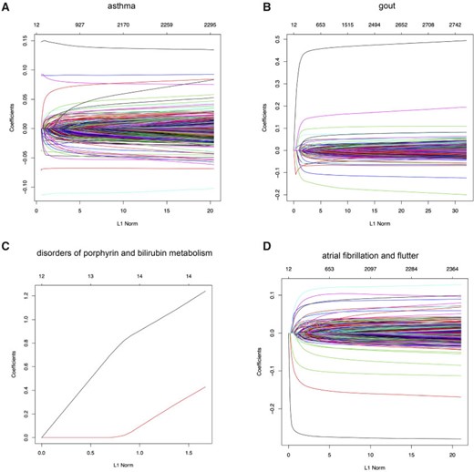
snpnet-Cox paths. Each line in these plots corresponds to a variable from the best model. The vertical axis represents the |$L^1$| norm of the estimated coefficients and the horizontal axis represents the value of the coefficients. The path is computed at various level of regularization parameter. The whiskers at the top of the plot are the number of variables selected. The first 12 variables are the covariates including age, sex, PC1-10.
We split our dataset into a |$70\%$| training (|$n = 236\,004$|), |$10\%$| validation, (|$n = 33\,716$|) and |$20\%$| held out test set (|$n = 67\,430$|), and apply snpnet-Cox with 50 iterations. We focus our analysis on 306 ICD10 codes with at least |$950$| cases in the |$337\,151$| individuals dataset.
3.3. snpnet-Cox results
We summarize the results across the 306 ICD10 codes, but focus our detailed analysis for four of them including:
asthma (ICD10 code: J45),
gout (M10),
disorders of porphyrin and bilirubin metabolism (E80), and
atrial fibrillation and flutter (I48).
The Lasso paths for these phenotypes are illustrated in Figure 1, where the estimated individual parameter values are plotted against the |$L^1$| norm of |$\hat{\beta}$|, for a decreasing sequence of |$\lambda$|. For an individual with genotype |$x$|, we define the Polygenic Hazard Score (PHS) to be |$\hat{\beta}^Tx$|, where |$\hat{\beta}$| is the fitted regression coefficients obtained from snpnet-Cox. We assess the predictive power of PHS on survival time using the individuals in the held out test set. We applied a couple of procedures to give a high-level overview of the results. First, we assessed whether the PHS was significantly associated to the time-to-event data in the held out test set (so that we obtained a |$\textit{P}$|-value for each ICD10 code). Second, we computed the hazards ratio (HR) for the scale (standard deviation unit), and different thresholded percentiles (top |$1\%$|, |$5\%$|, |$10\%$|, and bottom |$10\%$| compared to the 40–60|$\%$|) of |$\boldsymbol{X}\hat{\beta}$|. Third, we computed the C-index (Harrell and others, 1982).
The C-index for the |$101$| ICD10 codes with PHS |$\textit{P} < 0.01$| range from 0.511 to 0.884 (see Global Biobank Engine snpnet-Cox page https://biobankengine.stanford.edu/snpnetcox) and HR per standard deviation of PHS from 1.042 to 13.167. The results further highlight the sparsity property of Lasso in the Cox model implemented in snpnet-Cox with some ICD10 codes including a single active variable in the set and others with almost 2000 active variables (e.g., non-insulin-dependent diabetes mellitus).
3.3.1. Asthma - J45
Motivated by the varying age of asthma onset, a common disease that affects a substantial fraction of young adults, we hypothesized that a PHS could capture individuals that are not only at higher risk of disease onset but also at a higher risk of developing asthma at a younger age.
Here, we estimate a HR of 1.428 per SD of PHS (C-index of 0.605), and HR of 2.740, 2.137, and 1.825 for the top 1, 5, and 10|$\%$| of the PHS distribution compared to the 40–60%. Further, we find that |$14.2\%$| of individuals in the top |$1\%$| of the PHS score developed asthma by age 20.5 compared to only |$1.1\%$| in the bottom |$10\%$| and |$3.2\%$| of the 40–60 percentile of the PHS score (see Figure 2), which underscores the relevance of PHS in the context of early onset of common diseases that are hypothesized to have a monogenic signature (Kelsen and Baldassano, 2017). The asthma PHS is composed of 1.567 active variable of which some are known from previous Genome-Wide Association Studies (GWAS) of traits related to asthma. As an example, we identify the rs2381416 (MAF = 0.26) upstream of GTF3AP1 to associate with asthma with an effect size of |$-$|0.11. This variant has previously been found to associate with eosinophil count (Gudbjartsson and others, 2009) and severity of childhood asthma (Smith and others, 2017).
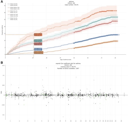
Asthma. (A) The Kaplan–Meier curves for percentiles of PHSs for variants selected by snpnet-Cox, in the held out test set (orange: top |$1\%$|, green: top |$5\%$|, red: top |$10\%$|, blue: 40-60|$\%$|, and brown: bottom 10|$\%$|; ticks represent censored observations. Highlighted are the proportion of asthma events by age 20 across the percentile scores. (B) Plot of snpnet-Cox coefficients for asthma with |$1567$| active variables. Green dots represent protein-altering variants.
3.3.2. Gout - M10
Gout is a common disease, affecting at least |$1\%$| of men in Western countries, with a strong male to female imbalance (Terkeltaub, 2003). It is a form of arthritis caused by excess uric acid in the bloodstream and characterized by severe pain, redness, and tenderness in joints.
In the UK Biobank study, we estimate a HR of 1.679 per SD of PHS (C-index of 0.649), and HR of 3.70, 2.502, and 2.073 for the top 1, 5, and 10|$\%$| of the PHS distribution compared to the 40–60%. Further, we find that |$4.89\%$| of individuals in the top |$1\%$| of the PHS score developed asthma by age 50.1 compared to only |$0.30\%$| in the bottom |$10\%$| and |$1.02\%$| of the 40–60 percentile of the PHS score (see Figure 3). The gout PHS consists of 1.970 active variables, and we identify loci that have been identified in prior GWAS (Dehghan and others, 2008).

Gout (A) The Kaplan–Meier curves for percentiles of PHSs for variants selected by snpnet-Cox, in the held out test set (orange: top |$1\%$|, green: top |$5\%$|, red: top |$10\%$|, blue: 40–60|$\%$|, and brown: bottom 10|$\%$|; ticks represent censored observations. Highlighted are the proportion of gout events by age 50 across the percentile scores. (B) Plot of snpnet-Cox coefficients for gout with |$1970$| active variables. Green dots represent protein-altering variants.
3.3.3. Disorders of porphyrin and bilirubin metabolism - E80
Bilirubin, which is the principal component of bile pigments, is the end product of the catabolism of the heme moiety of hemoglobin and other hemoproteins. If bilirubin is produced in excessive amounts or hepatic excretion of bilirubin into bile is defective, the concentration of bilirubin in the blood and tissues increases, which may result in jaundice (Bosma, 2003), a well-recognizable symptom of liver disease.
We estimate a HR of 13.167 per SD of PHS (C-index of 0.884). Here, given that we have only two active variables, we find that the snpnet-Cox algorithm finds a sparse solution (see Figure 4). One of the active variables is the intron variant (rs6742078) of UTG1A4 (MAF = 0.31) which encodes an enzyme (Uridine diphosphate) UDP-glucuronosyltransferase that transforms small lipophilic molecules such as bilirubin (Tukey and Strassburg, 2000).
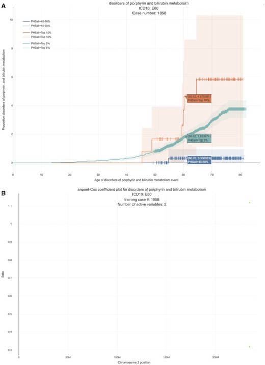
Disorders of porphyrin and bilirubin metabolism. (A) The Kaplan–Meier curves for percentiles of PHS for variants selected by snpnet-Cox, in the held out test set (orange: top |$1\%$|, green: top |$5\%$|, red: top |$10\%$|, blue: 40–60|$\%$|, and brown: bottom 10|$\%$|; ticks represent censored observations. Highlighted are the proportion of disorders of porphyrin and bilirubin metabolism events by age 60 across the percentile scores. (B) Plot of snpnet-Cox coefficients for disorders of porphyrin and bilirubin metabolism with |$2$| active variables. Green dots represent protein-altering variants.
3.3.4. Atrial fibrillation and flutter - I48
Atrial fibrillation is the most common type of arrhythmia in adults. The prevalence increases from less than |$1\%$| in persons younger than 60 years of age to more than |$8\%$| in those older than 80 years of age (McNamara and others, 2003). Earlier onset of atrial fibrillation is believed to have a strong genetic component and whether that has more of a polygenic or monogenic flavor is currently unknown.
In the UK Biobank study, we estimate a HR of 1.466 per SD of PHS (C-index of 0.618), and HR of 3.883, 2.319, and 1.861 for the top 1, 5, and 10|$\%$| of the PHS distribution compared to the 40–60%. Further, we find that |$6.57\%$| of individuals in the top |$1\%$| of the PHS score developed asthma by age 60 compared to only |$0.70\%$| in the bottom |$10\%$| and |$1.41\%$| of the 40–60 percentile of the PHS score (see Figure 5), which underscores the relevance of PHS in the context of early onset of atrial fibrillation.
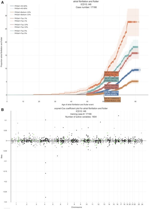
Atrial fibrillation. (A) The Kaplan–Meier curves for percentiles of PHSs for variants selected by snpnet-Cox, in the held out test set (orange: top |$1\%$|, green: top |$5\%$|, red: top |$10\%$|, blue: 40–60|$\%$|, and brown: bottom 10|$\%$|; ticks represent censored observations. Highlighted are the proportion of atrial fibrillation events by age 60 across the percentile scores. (B) Plot of snpnet-Cox coefficients for atrial fibrillation with |$1604$| active variables. Green dots represent protein-altering variants.
4. Discussion
In this article, we developed the batch screening iterative LASSO (BASIL) algorithm (Qian and others, 2019) to find the lasso path of Cox proportional hazard models. We implemented an optimized C-index function, which computes the C-index of a fitted Cox model in |$O(n \log n)$| time with an excellent constant factor. Our method was applied to the UK Biobank dataset to identify genetic variants that are associated with time-to-event phenotypes and to build PHS. Visualizations of snpnet-Cox results across 306 ICD10 codes are available in Global Biobank Engine (https://biobankengine.stanford.edu/snpnetcox) (McInnes and others, 2019).
Our current approach does have limitations, which we hope to resolve in future work. First, we assume that each individual has independent survival times (conditional on the features). This may become a limitation as population-scale cohorts especially in population isolates like in Finland sample related individuals. Second, we do not provide procedures to estimate the confidence intervals of the selected variables, which may be useful in communicating confidence in a single active variable (Taylor and Tibshirani, 2015). Third, as we move towards whole genome sequencing data where a large fraction of variants discovered will have a rare event property, i.e., observed in a handful of individuals, the validation accuracy may need to be redefined to evaluate a fitted |$\hat{\beta}$|. Fourth, we do not consider time-varying coefficients and time-varying covariates, which may improve inference in the setting where features may have multiple measurements over time. These are areas of future direction that we anticipate we will address.
5. Software
We provide the implementation of our approach in a publicly available package snpnet available at https://github.com/rivas-lab/snpnet with cindex package dependency available at https://github.com/chrchang/plink-ng/tree/master/2.0/cindex. The analysis results are published on figshare at https://figshare.com/articles/snpnet-Cox_results/12368294.
Supplementary material
Supplementary material is available at http://biostatistics.oxfordjournals.org.
Acknowledgments
Conflict of Interest: None declared.
Funding
Stanford University to R.L.; The Two Sigma Graduate Fellowship to J.Q., in part; Funai Overseas Scholarship from Funai Foundation for Information Technology and the Stanford University School of Medicine to Y.T. Stanford University and a National Institute of Health center for Multi and Trans-ethnic Mapping of Mendelian and Complex Diseases grant (5U01 HG009080) to M.A.R.; National Human Genome Research Institute (NHGRI) of the National Institutes of Health (NIH) under awards (R01HG010140). The content is solely the responsibility of the authors and does not necessarily represent the official views of the National Institutes of Health; NIH (5R01 EB001988-16) and NSF (19 DMS1208164) to R.T., in part; the National Science Foundation (DMS-1407548) to T.H., in part; The National Institutes of Health (5R01 EB 001988-21).
