


Summary
Our main goal is to study and quantify the evolution of multiple sclerosis lesions observed longitudinally over many years in multi-sequence structural magnetic resonance imaging (sMRI). To achieve that, we propose a class of functional models for capturing the temporal dynamics and spatial distribution of the voxel-specific intensity trajectories in all sMRI sequences. To accommodate the hierarchical data structure (observations nested within voxels, which are nested within lesions, which, in turn, are nested within study participants), we use structured functional principal component analysis. We propose and evaluate the finite sample properties of hypothesis tests of therapeutic intervention effects on lesion evolution while accounting for the multilevel structure of the data. Using this novel testing strategy, we found statistically significant differences in lesion evolution between treatment groups.
1. Introduction
Multiple sclerosis (MS) is an immune-mediated disease of the central nervous system. Structural magnetic resonance imaging (sMRI) is commonly used in patients with MS to monitor and manage the disease, quantify the location and volume of new lesions, and observe the dynamic changes of existing brain lesions. MS lesions appear hyperintense on some sMRI sequences (e.g., FLAIR, T2w) or hypointense on others (e.g., T1w) relative to normally appearing white matter (NAWM). Monitoring the dynamic changes in MS lesions can be conducted via longitudinal multimodal MRI collected at multiple visits. These processes are complex with a typical evolution of a lesion consisting of: (i) an initial phase when the lesion expands and is accompanied by inflammation of the surrounding tissue; (ii) a second phase when the lesion stabilizes in spatial extent and the inflammation is reduced; and (iii) a third phase, when the lesion slowly changes, with intensities of some areas remaining the same and intensities in other areas returning to values closer to those of NAWM. In some cases, the lesion can completely disappear from multimodal MRIs with the intensity of all lesion voxels returning to their corresponding baseline distributions in all sMRI sequences. In the work of Meier and Guttmann (2006) and Meier and others (2007), longitudinal lesion behavior was characterized using serial T2-weighted MRI. Ghassemi and others (2015) compared change over a 2-year period in T1 intensity within new T2 lesions between pediatric and adult-onset MS. More recently, Dworkin and others (2016) built a prediction model using imaging features, clinical information, and treatment status at the time of lesion incidence to predict voxel intensities approximately a year post-incidence. Here, we focus on quantifying the dynamic behavior of lesions in MS, which could be useful for clinical monitoring as well as a potential biomarker for studying the effect of treatments and predicting clinical outcomes.
In this article, we develop a general statistical model for quantifying MS lesion evolution using the individual trajectories of lesion voxel intensities in multiple sMRI sequences. We take a functional data perspective, where the observed voxel-specific longitudinal MRI intensities are viewed as discrete realizations of a continuous functional process. This makes sense as changes in lesions are expected to be continuous, while sMRIs are obtained at discrete time points during this continuous underlying biological process. We also develop a general hypothesis test for fixed effects in the resulting hierarchical functional model and apply it to test a treatment effect. We show that the proposed testing method is more powerful than a commonly used approach (where the hierarchical structure of the data is not taken into account) for testing for treatment effects in this sMRI setting.
The field of functional data analysis (FDA) has been under intense development due to the emergence of studies that collect functions or images as their sampling unit; an excellent monograph of FDA methods and techniques is provided by Ramsay and Silverman (2005). However, much of the FDA literature is focused on unstructured functional data, that is, when one independent functional measurement is sampled per unit. In contrast, structured functional data are focused on cases when the sample of functions has a known structure implied by the sampling mechanism. For example, Di and others (2009) introduced multilevel functional principal component analysis (MFPCA), the functional equivalent of multiway ANOVA, to account for repeated functional measurements within study participants. Zhou and others (2010) and Staicu and others (2010) extended MFPCA to multilevel functional data with spatial correlation, while Greven and others (2010) introduced longitudinal functional principal component analysis (LFPCA) for functions measured over time. LFPCA is a direct generalization of standard longitudinal mixed-effects models because the structure of the problem and data is the same as in longitudinal data analysis with the exception that the basic measurement is a function instead of a scalar at each visit. LFPCA provides a decomposition of longitudinal functional data into a time-dependent population average, baseline subject-specific variability, longitudinal subject-specific variability, subject-visit-specific variability, and measurement error. Unfortunately, both MFPCA (Di and others, 2009) and LFPCA (Greven and others, 2010) are infeasible in very high-dimensional settings, because they require the calculation and diagonalization of high-dimensional covariance operators. To address this problem, Zipunnikov and others (2011) proposed high-dimensional MFPCA and high-dimensional LFPCA, which share the same fundamental idea: (i) use a singular value decomposition of the data matrix and avoid calculating the covariance operators; (ii) project the data on the space spanned by the right singular vectors of the data matrix; and (iii) estimate the principal scores using Best Linear Unbiased Predictors (BLUPs). The method is computationally efficient, because the intrinsic dimension of the model is controlled by the sample size of the study instead of the number of voxels. Chen and Müller (2012) provided an alternative way for modeling longitudinal functional data. They proposed the double FPCA, which uses an initial FPCA at a grid of time points and then applies a second FPCA on the resulting principal components. More recently, Shou and others (2015) defined the class of structured functional models, which includes multi-way nested and crossed designs for functional data. Another group of commonly used approached for analyzing functional data includes wavelet-based functional mixed models (Morris and Carroll, 2006; Morris and others, 2006; Ciarleglio and Ogden, 2016). Staicu and others (2015) proposed hypothesis testing for group means in hierarchical functional data with spatial correlation. Covariance regularization in high dimensions has been widely studied in statistical literature. For instance, Bickel and Levina (2008) considered regularized estimation of large covariance structures by banding or tapering the sample covariance matrix. Fan and others (2013) proposed estimation of large covariance matrices by thresholding principal orthogonal complements.
However, modeling the dynamic process of changes in the voxel intensities in MS lesions raises methodological challenges that have not been addressed yet. For example, MS lesions can occur at any time during the disease process and at various locations in the brain. Therefore, the data are unbalanced both in time and space, while the number of visits varies across subjects and lesions. This happens because some lesions occur earlier than others, and newer lesions are observed at fewer time points. Moreover, we have multiple sMRI sequences, and voxels are spatially correlated within lesions. To address these challenges, we develop a structured functional model that characterizes the known sources of variation in the dynamics of multi-sequence voxel intensities during the lesion development process. In the context of this model, we also propose hypothesis tests on the effects of therapeutic interventions on lesion evolution, while accounting for the multilevel structure of the data.
Our work continues and expands the models developed by Sweeney and others (2015), who proposed to convert the multi-sequence longitudinal voxel intensity profiles into a biomarker using principal component analysis (PCA). While this approach proved to be very useful, some information is lost by ignoring the within-lesion and within-person structure of the intensity profiles. We also show that accounting for this multilevel structure can improve the performance of our novel testing procedure. Our testing approach extends ANOVA testing procedures (Zhang and Grossmann, 2016; Zhang, 2013) to structured functional data.
2. Models and framework
2.1. Data
We started with images from 60 patients with MS who were scanned between 2000 and 2008 on a (approximately) monthly basis for a certain period of time during the 8-year period at the National Institutes of Health Clinical Center in Bethesda, Maryland. The patients were followed for a range from 0.9 to 5.5 years (mean = 2.2, SD = 1.2). We only included study participants whose data satisfied the following inclusion criteria: (i) the study participant has at least one new lesion during the follow-up; (ii) the study participant has a scanning visit at least once within 100 days after lesion incidence; and (iii) all scans for the study participant passed a visual quality control, checking for the quality of the automated lesion segmentation. This reduced the sample size from 60 to 36 study participants. Among the 36 study participants left in our sample, 21 were female and 15 were male. The baseline age of the study participants was between 18 and 60 years, with a mean of 37 years (SD = |$9.6$|). Thirty-one study participants had relapsing-remitting MS and five had secondary-progressive MS. The study participants were either untreated or treated with various disease-modifying therapies that included both FDA-approved and experimental treatments changing over the course of data collection. Seven study participants received steroids during the course of the study.
Image acquisition and preprocessing details have been published by Sweeney and others (2015). Here, we provide a short summary for completeness of discussion. Whole-brain 2D FLAIR, PD, T2, and 3D T1 volumes were acquired on a |$1.5$| T MRI scanner (SIGNA Excite HDxt; GE Healthcare, Milwaukee, WI, USA). A body coil was used for transmission and a head coil as receiver. The 3D T1 volume was acquired using a gradient-echo sequence, and the 2D FLAIR, PD, T2 volumes were acquired using fast-spin-echo sequences. Short and long echoes from the same sequence were used to acquire the PD and T2 volumes. Medical Image Processing Analysis and Visualization (http://mipav.cit.nih.gov) and the JAVA Image Science Toolkit (http://www.nitrc.org/projects/jist) were used for image preprocessing (Lucas and others, 2010). Each image was interpolated to a voxel size of 1 mm|$^3$| and rigidly co-registered to a template space across time and across sequences (Fonov and others, 2009). After removing the extracerebral voxels using a skull-stripping procedure (Carass and others, 2007), the brain was automatically segmented using the Lesion-TOADS algorithm to produce a mask of NAWM (Shiee and others, 2010), which does not include white matter lesions. Since MRI data are acquired in arbitrary units, statistical normalization was applied to image intensities (Shinohara and others, 2011, 2014). Lesions at the baseline visit were obtained using the OASIS automatic algorithm for lesion segmentation (Sweeney and others, 2013b). The lesions identified at the baseline visit were removed from the analysis as their incidence time was unknown. Lesions at subsequent visits were segmented using the SubLIME method (Sweeney and others, 2013a). The true lesion incidence time would be a time point between the first scan where the lesion was identified by the SubLIME method (used as lesion incidence time in our analysis) and the previous time where the lesion did not appear.
2.2. Functional PCA for modeling lesion intensities
One of the inherent assumptions in our modeling approach is that images have been longitudinally co-registered (registered within person); registration to a common template was not necessary. Longitudinal co-registration was necessary to track the voxel intensities longitudinally and ensure that they have the same interpretation at every visit. For the purpose of this article, we assume there are no registration errors. Sweeney and others (2015) provided evidence that the distance between the voxel and the lesion boundary is strongly associated with changes in sMRI intensity over time. Therefore, voxels are first grouped within the same lesion by their distance to the boundary. We call these groups of voxels “lesion layers.” The number of layers within the lesion varies depending on its size. We define the layers of a particular lesion at the time of lesion incidence. The layers do not change even if the boundary of the lesion may change over time. Figure 1 shows a lesion where each voxel is colored by its distance to the lesion boundary. Voxels with the same color are in the same layer.
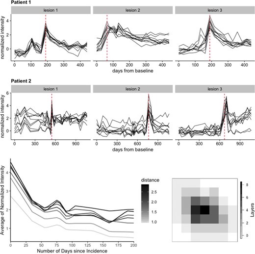
Top 2 rows: lesion trajectories over time for three lesions randomly selected from two participants in the study. Here, 10 voxels are randomly chosen from each lesion to illustrate the intensity trajectories of the lesion voxels (in black) during the full course of the study. The red dotted line shows the lesion incidence time for each lesion within the full study duration for each of the two participants. Bottom row: intensity trajectories averaged across each lesion layer and colored by the distance of that layer from the lesion boundary (left). These trajectories correspond to the lesion presented on the right. A 2D slice from a lesion where each voxel is colored by its distance to lesion boundary (right). Layer 0 does not contain lesion voxels.
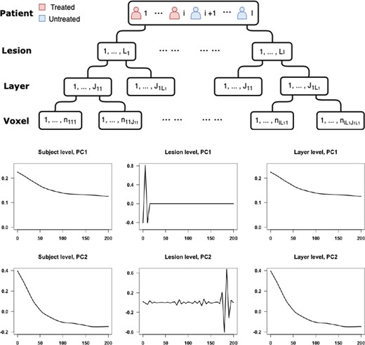
Top: display of the hierarchical structure of the data. Bottom: the first two principal components for subject-, lesion-, and layer-levels estimated by the SFPCA model.
2.3. Functional PCA with nested design
2.4. Covariance estimation
Therefore, the estimated covariance matrices |$\hat{K}_W = \dfrac{1}{2} \hat{H}_W = \mathbf{YG_WY^T}$|, |$ \hat{K}_U = \dfrac{1}{2} (\hat{H}_U-\hat{H}_W) = \mathbf{YG_UY^T}$| , and |$ \hat{K}_X = \dfrac{1}{2} (\hat{H}_X-\hat{H}_U)= \mathbf{YG_XY^T} $| all can be written in the form of |$\mathbf{Y}\mathbf{G}\mathbf{Y}^T$|. It is easy to show that the estimators are unbiased in finite samples given their straightforward methods of moments construction.
2.5. Data with noise
So far, we have ignored the case when |$\sigma^2>0$|, though in many applications the residual variability can be substantial. This problem can be addressed by smoothing the covariance matrix estimators or the raw data (Shou and others, 2015). Shou and others (2015) stated difficulties that could occur when applying the approach of smoothing covariance matrix estimators to high-dimensional functional data. First, when |$p \geq 10,000$|, it is not computationally feasible to conduct the bivariate smoothing on the |$p \times p$| covariance matrix. Second, when projected onto the lower-dimensional space, the one-to-one mapping of the eigenvalues and principal scores no longer holds after smoothing. Therefore, Shou and others (2015) recommend smoothing the raw data before conducting SFPCA. We use this latter approach in our application.
2.6. Analysis of MS lesion profiles
We treat each voxel as the basic unit of observation. We are interested in modeling the normalized MRI intensities of the voxel over time. Voxels are naturally nested within lesions, which are further nested within subjects; this provides a natural multilevel structure for the functional data with a minimum of three levels. To provide a visual representation of the intensity profiles over time, Figure 1 displays the intensity trajectory from T2 sequencing for 10 voxels for each of 3 lesions from 2 study participants. The rows of panels in Figure 1 correspond to subjects and the columns correspond to lesions. Time on the |$x$|-axis corresponds to time from entry into the study of that particular study participant. The y-axis in every panel corresponds to normalized intensities relative to NAWM (Shinohara and others, 2014); for example, |$-1$| represents minus one standard deviation (of the intensities of the NAWM voxels) away from the mean of the NAWM. This makes units comparable within- and between-lesions. The vertical red dash line in each panel indicates when the lesion was first detected.
Before applying functional principal component analysis (FPCA), we pre-process the data. First, we group the voxels within the same lesion by their distance to the boundary as lesion layers and compute the mean intensities within each layer at each time point. Data are then aligned to ensure that time 0 is incidence time. We linearly interpolate intensities in 5-day intervals over the 200-day period after lesion incidence. Therefore, each layer within a lesion has a single (average) intensity value for each of the |$p = 41$| time points 5 days apart. Figure 1 displays the trajectories of the layer-specific mean intensities for a randomly sampled lesion after pre-processing along with the lesion’s layer structure on the right side as a reference. Darker shades of gray correspond to larger distance to the boundary, while lighter shades correspond to smaller distances. Distances here are expressed as number of voxels between the layer and the boundary of the lesion using the shortest distance.
After smoothing and demeaning the intensities, we estimate the covariance functions for subject-, lesion-, and layer-levels and apply SFPCA to estimate eigenvalues for each of the levels of the model. The eigenvalues show that the first principal component at every level explains 96.5% of the level-specific variability. Among the levels, subject level |$(X)$| only explains 2.5% of the variability, while the lesion level |$(U)$| explains 50% of the variability and the layer level |$(W)$| explains 47.5% of the variability. The first and second principal components for each level are plotted in Figure 2.
2.7. Interpretation of principal components
The first principal component for the layer-specific process |$W_{ilj}(t)$| accounts for the change in intensity over time. At the lesion level, there is a large and rapid variation close to lesion incidence time, which does not have an obvious interpretation. We consider two possible sources of the variation that would result in the observed shape of the lesion-level PC and evaluate each of the two hypothesized sources by simulations. One possible source of variation is the uncertainty in the true lesion incidence time. The lesion incidence happens at any time point between the scan where we first observe the lesion and its previous scan. We use the time when we observe the lesion as an estimate of lesion incidence time. This results in variability of the time point when we first observe the lesion intensity trajectory across lesions and participants, possibly causing the observed shape of the lesion-level PC. The other hypothesized source of variability is the difference between scanning frequency across subjects and within subjects (i.e., across lesions within a subject). While approximately monthly scans were available for all subjects in the study, there was a variability of about |$\pm5$| days among monthly scanning visits for study participants. To evaluate the effects of these two sources of variability using simulation studies, we generate data from the following true model.
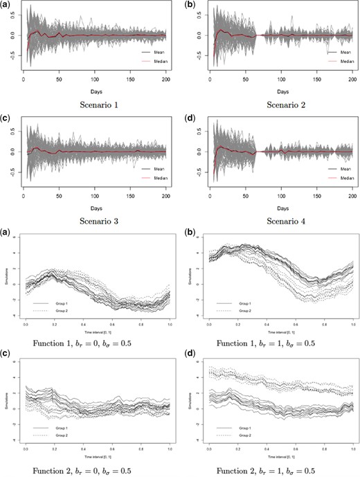
Top 2 rows: first principal component at the lesion level estimated under four different scenarios of data collection. Each gray line corresponds to the lesion-level PC1 estimated within a single simulation run out of 100. The black and red lines correspond to the median and mean trajectories of the 100 PC1 estimates, respectively. Bottom 2 rows: illustrations of the functional forms and the corresponding parameters using to generate data for the four simulation scenarios.
3. Hypothesis testing
3.1. Analysis of variance
To construct the test statistic for these hypotheses, we start by extending the idea of analysis of variance to the functional setting. Table 1 provides the variance apportioning by source for a given time, |$t$|, where |${\rm SS}(t)$| denotes the sum of squares for a given time point, |$t$|. Notation is canonical, where |$\bar{y}_{....}(t)$| is the overall mean, |$\bar{y}_{g...}(t)$| is the mean over observations in group |$g$|, |$\bar{y}_{gl..}(t)$| is the mean over observations in lesion |$l$| within group |$g$|, etc. We consider the case of a balanced design with the same number of sub-levels on each level. This simplifies notation substantially, for example, Table 1a becomes Table 1b and also guarantees a closed form of expected mean squares, which are displayed in Table 1c.
Details on analysis of variance
| a. Analysis of variance table | ||
|---|---|---|
| Source | df | SS(t) |
| Group | |$G - 1 $| | |$\sum_{g=1}^G\sum_{l = 1}^{L_g} \sum_{j = 1}^{J_l}\sum_{v = 1}^{V_j} (\bar{y}_{g...}(t) - \bar{y}_{....}(t))^2$| |
| Lesion | |$\sum_{g =1}^G (L_g - 1)$| | |$\sum_{g=1}^G\sum_{l = 1}^{L_g} \sum_{j = 1}^{J_l} \sum_{v = 1}^{V_j} (\bar{y}_{gl..}(t) - \bar{y}_{g...}(t))^2$| |
| Layer | |$\sum_{g =1}^G \sum_{l = 1}^{L_g} (J_l - 1)$| | |$\sum_{g=1}^G\sum_{l = 1}^{L_g} \sum_{j = 1}^{J_l} \sum_{v = 1}^{V_j} (\bar{y}_{glj.}(t) - \bar{y}_{gl..}(t))^2$| |
| Error | |$\sum_{g =1}^G \sum_{l = 1}^{L_g} \sum_{j = 1}^{J_l}(V_j - 1)$| | |$\sum_{g=1}^G\sum_{l = 1}^{L_g} \sum_{j = 1}^{J_l} \sum_{v = 1}^{V_j} (\bar{y}_{gljv}(t) - \bar{y}_{glj.}(t))^2$| |
| b. Analysis of variance table (simplified) | ||
| Source | df | SS(t) |
| Group | |$G 1$| | |$\sum_{g=1}^G LJV (\bar{y}_{g...}(t) - \bar{y}_{....}(t))^2$| |
| Lesion | |$ G (L - 1)$| | |$\sum_{g=1}^G\sum_{l = 1}^{L} JV (\bar{y}_{gl..}(t) - \bar{y}_{g...}(t))^2$| |
| Layer | |$G L (J - 1)$| | |$\sum_{g=1}^G\sum_{l = 1}^{L} \sum_{j = 1}^{J} V (\bar{y}_{glj.}(t) - \bar{y}_{gl..}(t))^2$| |
| Error | |$GLJ(V - 1)$| | |$\sum_{g=1}^G\sum_{l = 1}^{L} \sum_{j = 1}^{J} \sum_{v = 1}^{V} (\bar{y}_{gljv}(t) - \bar{y}_{glj.}(t))^2$| |
| c. Expected mean square errors | |
|---|---|
| Source | EMS(t) |
| Group | |$ JVL\frac{\sum_{g = 1}^2 \tau_{g}(t)^2}{2-1}+ JVK_{U}(t,t) + V K_W(t,t) + K_{\epsilon}(t,t)$| |
| Lesion | |$JVK_{U}(t,t) + V K_W(t,t) + K_{\epsilon}(t,t)$| |
| Layer | |$ V K_W(t,t) + K_{\epsilon}(t,t) $| |
| Error | |$ K_{\epsilon}(t,t) $| |
3.2. F-type test for main effect
The |$I$| samples are |$X_1(t), X_2(t), \dots, X_I(t) \in \mathcal{L}^2(\mathcal{T})$|, where |$\mathcal{L}^2(\mathcal{T})$| denotes the Hilbert space that is formed by all squared integrable functions with support in |$\mathcal{T}$|, and |$tr(K_X) < \infty$|.
The |$I$| samples are drawn from a Gaussian process.
As |$n \longrightarrow \infty$|, the |$I$| sample sizes satisfy |$n_{i\cdot}/n \longrightarrow \tau_i$|, such that |$\tau_1, \tau_2, \dots, \tau_I \in (0,1)$|.
The lesion-effect function |$U_{il}(t)$| and layer-effect function |$W_{ilj}(t)$| are i.i.d., where |$i = 1, 2, \dots, I$|,|$l = 1, 2, \dots, L_i$|, and |$j = 1, 2, \dots, J_{il}$|.
we obtain
where |$U_r$| are independent, |$U_r\sim \chi^2_{n-1}$|, |$ \theta_1, \dots, \theta_{\infty} $| are the eigenvalues of the covariance operator |$ \delta(\cdot,\cdot) $| and |$ \bar{x}(t) = \dfrac{1}{n}\sum_{i = 1}^n x_i(t)$|.
3.3. Simulation studies to evaluate the power of the proposed test
We compared our approach with the mixed-effects model testing approach used by Sweeney and others (2015). More specifically, we used the model |$Y_{gljv}(t) = \mu(t)+\tau_g(t) + U_{gl}(t) + W_{glj}(t) + \epsilon_{gljv}(t)$| and the F-type test statistic |$F = \dfrac{\int_{\mathcal{T}} SS_{\rm Group}(t){\rm d}t/ {\rm d}f_{\rm Group}}{\int_{\mathcal{T}} SS_{\rm Lesion}(t){\rm d}t/ {\rm d}f_{\rm Lesion}}$| as specified in Section 3.2. When using the mixed-effect model, the longitudinal trajectory of intensity is converted to a single value biomarker and used as the response of the model. The size-corrected power (Lloyd, 2005) of the two tests are compared in Table 2 using 1000 simulations. When judging a test, the standard approach is to maximize power, while limiting size by a pre-specified significance level |$\alpha^*$|. However, the actual size of the test |$\alpha$| may be different from the target significance level. Comparing the powers of two competing tests with unequal sizes is meaningless. To ensure there is no size distortion, the critical values may need to be altered up or down from the one that is associated with the nominal significance level. The new critical value used in computing the size-corrected power is usually obtained by conducting Monte Carlo simulation, for example, the critical value is 2.216 for function (1), |$b_{\tau} = 0.5$|. We observe that the size-corrected power of our proposed testing procedure increases as the difference between the two groups increases. Comparing to the mixed-effect model, our proposed test has a higher size-corrected power than the competitor approach in all simulation scenarios. We conclude that treating the response as functional data while accounting for the multilevel improves the performance of the testing procedure.
Size-corrected power
| Function 1 | Function 2 | ||||
|---|---|---|---|---|---|
| |$b_{\tau}$| | |$b_{\sigma}$| | Hierarchical HT | Mixed-effect model | Hierarchical HT | Mixed-effect model |
| 0 | 0.5 | 0.06 | 0.05 | 0.06 | 0.04 |
| 0 | 1 | 0.05 | 0.04 | 0.05 | 0.05 |
| 0.1 | 0.5 | 0.42 | 0.28 | 0.41 | 0.27 |
| 0.1 | 1 | 0.49 | 0.28 | 0.42 | 0.27 |
| 0.2 | 0.5 | 0.95 | 0.55 | 0.95 | 0.53 |
| 0.2 | 1 | 0.98 | 0.51 | 0.97 | 0.54 |
| 0.5 | 0.5 | 1 | 0.62 | 1 | 0.62 |
| 0.5 | 1 | 1 | 0.60 | 1 | 0.62 |
| 1 | 0.5 | 1 | 0.72 | 1 | 0.75 |
| 1 | 1 | 1 | 0.74 | 1 | 0.72 |
3.4. Testing for treatment effect
We grouped participants in the NIH-based study that received any disease-modifying treatments into a treatment group and those on no treatments in an untreated group. There were 290 lesions in the treated group and 179 lesions in the untreated group. The lesion size is quite heterogeneous, with a median number of layers equal to 5 (SD = 4.92, min = 1, max = 30). In addition, the lesion layers have highly variable number of voxels, while outer layers have more voxels than the inner layers. In order to apply our proposed hypothesis testing procedure, we further pre-process the data to obtain a balanced design in terms of the lesion-, layer-, and voxel-levels. In other words, we assume that each level has the same number of sub-levels. At the group level, we randomly select 179 lesions from the treated group, yielding the same number of lesions in treated and untreated groups. For the lesion- and layer-levels, we use a combination of subsampling and bootstrapping to ensure that each lesion includes five layers and each layer includes 10 voxels. For example, if a lesion has eight layers, we randomly sample five layers without replacement, while if a lesion has three layers, we randomly sample two additional layers with replacement. The same method is applied to layer level. The proportion of lesions and layers that needed to be upsampled or downsampled were approximately the same within the treated and untreated groups. The null hypothesis we are interested in testing is that there is no treatment effect, while the alternative hypothesis states that there is treatment effect. After applying the F-test, we obtain the test statistics |$F = 8.45$|, with p-value |$= 0.002$|. The null hypothesis is rejected at |$\alpha = 0.05$| implying that there is a significant difference in lesion evolution between treated and untreated groups. This finding is consistent with the literature on this topic (e.g., Sweeney and others, 2015).
4. Discussion
We propose a structured functional model that characterizes the dynamic process of changes in voxel intensities in MS lesions. Challenges raised by the MS lesion data are the hierarchical structure and the unbalanced data collection scheme in both space and time. We preprocess data by aligning the trajectories by their incidence time, extracting available scanning visit data within 200 days post-lesion incidence, and extrapolating lesion intensities on a 5-day grid. As a result, we obtain a sampling scheme where each lesion is observed for the same length of time after incidence with the same frequency. We apply the SFPCA method to model the data to allow for a robust decomposition of the observed functional variability at lesion-, layer-, and subject-levels. We obtain that the lesion level explains 50% of the variability, layer level explains 47.5% of the variability, and subject level explains only 2.5% of the variability. This result indicates that MS lesion evolution is relatively homogeneous at the subject level. Hence, we remove the subject level effects from further analysis. Within levels, the first principal component at every level explains 96.5% of the level-specific variability. While the first PC over time on layer level coincides with the trend of lesion intensity trajectory, the interpretation of first PC on lesion level is not so obvious. We develop a simulation study approach to identify possible interpretations for the shape of this estimated PC. Specifically, we add different sources of variation gradually in simulations to identify the possible interpretation.
In the second part of the study, we propose a hypothesis testing procedure for no effect of therapeutic interventions on lesion evolution, while accounting for the hierarchical structure of the data. We extend the idea of analysis of variance to the functional setting and apply it to data with balanced design, that is to the case when there is an equal number of sub-levels on each level. This substantially simplifies notation and provides a closed form of the distribution of the F-type test statistics. We compare the performance of the proposed method to that of a mixed-effect model using simulation studies. The proposed hierarchical hypothesis has a higher size-corrected power in all the scenarios. We apply the hierarchical hypothesis testing to the MS lesion data after balancing the data by subsampling and bootstrapping. We show that there is sufficient evidence to reject the null hypothesis of no treatment effect. Our study indicates that the lesion evolution process is significantly different between participants on disease-modifying treatments and those that are untreated.
One limitation of our study is that both SFPCA and hierarchical hypothesis testing have not been studied in the case of unbalanced data. While SFPCA can be applied to unbalanced observational data, the estimation of covariance becomes complicated. In hypothesis testing, the calculation also becomes challenging for unbalanced data. In addition, the expected mean square errors cannot be expressed in closed form, while the distribution of the test statistic computed using (3.7) under the null hypothesis may not belong to a family of known distributions. Future studies may consider the theoretical aspects of determining the distribution of the test statistic or investigate the empirical distribution of the proposed test statistic under unbalances design settings or using a permutation testing approach. In addition, when p is large (|$p > 10\,000$| or |$p>>n$|), the model needs to be mapped onto a lower-dimensional space (Zipunnikov and others, 2011) to avoid calculating the covariance operators in the original p-dimensional space. Further exploration of the application to unbalanced data remains an open problem. Future studies may also consider simulating the null distribution directly without using the F-distribution approximation. Another limitation of our study is the assumption that the noise in (2.1) has a Gaussian distribution. Preliminary residual analysis for the MS data example presented in our paper showed that while the distribution of estimated residuals is approximately symmetric, it has heavier tails than the Gaussian density. Future studies may generalize this model by incorporating more general distributional assumptions for the noise component |$\sigma^2$| in (2.1).
Software
Software for performing hypothesis testing procedures presented in our article is available via GitHub through the following URL: https://github.com/mhnaomi/fpca_paper.
Acknowledgments
Conflict of Interest: None declared.
Funding
The National Institutes of Neurological Disorders and Stroke (NINDS) (R21 NS093349); and the National Institute of General Medical Sciences (5P20GM103645), in part. Intramural Research Program of NINDS, in part. The content is solely the responsibility of the authors and does not necessarily represent the official views of the funding agencies.
