


Summary
A dynamic treatment regimen (DTR) is a sequence of decision rules that can alter treatments or doses based on outcomes from prior treatment. In the case of two lines of treatment, a DTR specifies first-line treatment, and second-line treatment for responders and treatment for non-responders to the first-line treatment. A sequential, multiple assignment, randomized trial (SMART) is one such type of trial that has been designed to assess DTRs. The primary goal of our project is to identify the treatments, covariates, and their interactions result in the best overall survival rate. Many previously proposed methods to analyze data with survival outcomes from a SMART use inverse probability weighting and provide non-parametric estimation of survival rates, but no other information. Other methods have been proposed to identify and estimate the optimal DTR, but inference issues were seldom addressed. We apply a joint modeling approach to provide unbiased survival estimates as a mechanism to quantify baseline and time-varying covariate effects, treatment effects, and their interactions within regimens. The issue of multiple comparisons at specific time points is addressed using multiple comparisons with the best method.
1. Introduction
Many diseases, chronic and acute, require sequences or combinations of treatments. Multiple first- and second-line treatment options are available for many diseases, but most of the evidence for best treatment focuses on treatments at one particular time in the treatment or disease process. To be useful for clinicians and patients, treatment guidelines should encompass the whole treatment regimen and provide sequences of decision rules at each stage of clinical intervention based on efficacy outcomes from earlier treatments. A dynamic treatment regimen (DTR) (Murphy and others, 2001) is one such sequence of decision rules. In the case of two lines of treatment, a DTR includes a first-line treatment, a second-line treatment for responders to that first-line treatment, and a second-line treatment for nonresponders to that first-line treatment. For diseases and disorders where DTRs are standard practice, evidence for optimal clinical decision rules considering more than one stage of treatment is necessary. A sequential, multiple assignment, randomized trial (SMART) (Murphy, 2005, Lavori and others, 2000, Lavori and Dawson, 2004) is one type of trial designed to assess entire treatment regimens to build effective DTRs. In such a multi-stage trial, second-line treatment may be randomized based on a patient’s outcome to a first-line treatment. DTRs are embedded within a SMART for estimation and comparison. The goal of a SMART is to identify decision rules or DTRs that result in the best overall outcome.
Figure 1 shows three of the most common two-stage SMART designs. In Design I, there are eight embedded DTRs: {|$A_1B_1C_1$|}, {|$A_1B_1C_2$|}, {|$A_1B_2C_1$|}, {|$A_1B_2C_2$|}, {|$A_2B_1C_1$|}, {|$A_2B_1C_2$|}, {|$A_2B_2C_1$|}, and {|$A_2B_2C_2$|}, where each set consists of a first-stage treatment (|$A_1$| or |$A_2$|), a second-stage treatment for responders (|$B_1$| or |$B_2$|), and a second-stage treatment for non-responders (|$C_1$| or |$C_2$|). Examples of SMARTs using this design include Fu and others (2017), Kelleher and others (2017), and Kim and others (2019). Note that every observed subject is consistent with two DTRs (e.g. those who receive the treatments |$A_1$| followed by |$B_1$| are consistent with two DTRs {|$A_1B_1C_1$|} and {|$A_1B_1C_2$|}; similarly, those who receive treatments |$A_1$| followed by |$C_1$| are consistent with {|$A_1B_1C_1$|} and {|$A_1B_2C_1$|}, etc.) This feature of a SMART allows for efficient use of each subject’s information to estimate the DTR outcome (Ko and Wahed, 2012). Design II is a variation of a SMART design where second-line treatments are only assigned to responders, resulting in four DTRs: {|$A_1B_1C_1$|}, {|$A_1B_2C_1$|}, {|$A_2B_1C_1$|}, and {|$A_2B_2C_1$|}. Examples of SMARTS using this design include Auyeung and others (2009), Naar and others (2019), and Schmitz and others (2018). Design III has second-line treatments only for responders from |$A_1$|, resulting in three DTRs |$\{A_1B_1C_1\}$|, |$\{A_1B_2C_1\},$| and |$\{A_2B_1C_1\}$|. Examples of SMARTs using this design includes Ruppert and others (2019) and Almirall and others (2016). Note that “response” and “non-response” may be switched in different contexts (e.g. non-responders may receive second treatment while responders maintain their first-line treatment or stop), but this change is trivial. Other SMART designs exist with different numbers of stages and treatments.
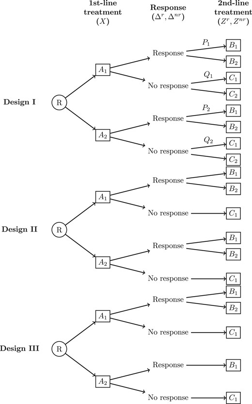
Three common two-stage sequential, multiple assignment, randomized trial (SMART) designs. R denotes the first randomization to first-line treatment |$A_1\:(X=0)$| or |$A_2\:(X=1)$|. |$\Delta^r$| and |$\Delta^{nr}$| are indicators of responders and non-responders to first-line treatment, respectively. |$B_1 \:(Z^r=0)$| and |$B_2\:(Z^r=1)$| are second-line treatment options for responders. |$C_1\:(Z^{nr}=0)$| and |$C_2\:(Z^{nr}=1)$| are second-line treatment options for non-responders. |$P_j=P(Z^r=1\mid A_j)$| and |$Q_j=P(Z^{nr}=1\mid A_j)$| are second-line randomization probabilities after treatment |$A_j$|, |$j=1,2$|. In design I, both responders and non-responders are re-randomized to second treatment. In design II, only responders are re-randomized. In design III, only responders from |$A_1$| are re-randomized.
Survival outcomes have been assessed in SMART literature. Many survival estimators have been built upon the inverse probability weighting (IPW) framework (Lunceford and others, 2002), with variations include time-dependent IPW (Guo and Tsiatis, 2005), modified supremum weighted log-rank test (Feng and Wahed, 2008), weighted Kaplan–Meier estimator (Miyahara and Wahed, 2010), and cumulative incidence function for competing risks (Yavuz and others, 2018), among others (Wahed, 2010, Feng and Wahed, 2009, Li and Murphy, 2011). These methods estimate DTRs’ averaged survival outcomes, but do not offer a way to parameterize treatment effects, interactions, or incorporate auxiliary variables (i.e. baseline covariates and those measured up to second-stage randomization).
Methods that do incorporate auxiliary variables extend the standard Cox model. Lokhnygina and Helterbrand (2007) incorporated IPW into a Cox model to compare separate-path DTRs (e.g. DTRs with different first-line treatment such as {|$A_1B_1C_1$|} and {|$A_2B_1C_1$|} in design II), but could not compare shared-path DTRs (Kidwell and Wahed, 2013) (e.g. DTRs with the same first-line treatment such as {|$A_1B_1C_1$|} and {|$A_1B_2C_1$|} in design II). Thall and others (2007) proposed a Bayesian joint model that regressed the overall survival time on intermediate response time, but assumed a rather restrictive Weibull distribution for both time points. Tang and Wahed (2015) assigned different Cox baseline hazards for each DTR and modeled auxiliary variables as covariate effects on the hazard ratios. This approach used different baseline hazards to represent the overall difference between DTRs but does not offer a way to measure each treatment’s effect and their interaction within DTRs. Moreover, they assumed that the auxiliary covariates’ effects were constant over different treatment stages within each DTR and across different DTRs. Zhao and others (2014) and Díaz and others (2018) introduced doubly robust estimation methods of the optimal individualized treatments for the survival data, but these methods can only be applied to one-stage treatment. Jiang and others (2017) proposed another doubly robust estimation method that could potentially be used for two-stage DTRs, but the time to assign treatments needs to be pre-specified, which is generally not feasible in the SMART setting with a survival outcome because treatments are usually assigned immediately after the responses are observed. Hager and others (2018) proposed a method to identify and estimate the optimal DTR in a SMART or observational study setting. However, their method could not make inference on which treatments, covariates or interactions contribute to the optimal DTR.
In this manuscript, we propose a joint modeling approach that looks at time-to-response and time-to-death in the context of survival data from a SMART. This approach has been used to model time to various stages in cancer patients (Tran and others, 2018). The joint model offers a way to measure first- and second-line treatments within a regimen and their interactions while naturally adjusting for randomization probabilities. Unless otherwise stated, the notation and simulation results are based on design II. As we will show, adaptation to design I and III is straightforward (see Section C.2 of the Supplementary material available at Biostatistics online for simulation result of Design I). In Section 2, we introduce the method including notation for a SMART with a survival outcome (Section 2.1), the proposed model (Section 2.2), the joint log-likelihood (Section 2.3), and non-parametric maximum likelihood estimator (NPMLE) (Section 2.4). Section 3 presents Monte Carlos simulations, which includes estimation performance (Section 3.1) and comparisons with other SMART time-to-event endpoint methods (Section 3.2). Since many pairwise DTR comparisons may be made to find the best DTR in a SMART, we also tackle the issue of multiple comparisons. In Section 4, we implement multiple comparisons with the best (MCB) to compare survival rates at some time |$t$| between DTRs. In Section 5, we apply the method to a trial to estimate the survival probabilities of DTRs and conclude with a discussion (Section 6).
2. Methods
2.1. Notation for SMARTs data structure
|$T^{r}$|, |$T^{d}$|, and |$T^{c}$| are potentially observed first-line response time, overall survival time, and censoring time, respectively. If a patient does not respond by |$t^{nr}$| or dies first, |$T^{r}$| is not observed. Thus, we can relate the first observed event time as |$T_1=\min(T^{r}, t^{nr}, T^{d}, T^{c})$|. Indicators |$\Delta^{r}={\rm 1}\kern-0.24em{\rm I}(T^{r}=T_1)$| and |$\Delta^{nr}={\rm 1}\kern-0.24em{\rm I}(t^{nr}=T_1)$| denote whether the patient is a responder or non-responder, respectively. Note that |$\Delta^{r}+\Delta^{nr}=0$| indicates that a patient was censored or died before the response assessment to first-line treatment. If |$\Delta^{r}+\Delta^{nr}=1$|, a patient is re-randomized to receive a second-line treatment. Subsequent survival time or censoring time is observed at |$T_2=\min(T^{d}, T^{c})$|. The indicator |$\Delta^{d}={\rm 1}\kern-0.24em{\rm I}(T^d=T_2)$| denotes that a death is observed.
2.2. Model
Note that in design II, all regimens have |$Z^{nr}=0$|, thus its effect is absorbed into the baseline hazards. For ease of notation, we denote |$\theta=e^{\beta_{1}V+\beta_{2}X}$|, |$\gamma=e^{\beta_{3}V+\beta_{4}X}$|, |$\eta=\gamma e^{\beta_{5}+\beta_{6}X+\beta_{7}Z^r+\beta_{8}XZ^r+\beta_{9}XZ^rV}$|, and |$\mu=\gamma e^{\beta_{10}+\beta_{11}X}$|. Denote |$S(t)$| and |$f(t)$| as the corresponding survival and density functions, respectively, for hazard functions |$\lambda(t)$|.
The current form of (2.2) can easily be adapted for designs I and III as follows:
Design I |$\lambda_{d}(t)\,{=}\,h_{d}(t)\exp \lbrace \beta_{3}V+ \beta_{4}X+ {\rm 1}\kern-0.24em{\rm I}(t>t^r<t^{nr})(\beta_{5}+\beta_{6}X+\beta_{7}Z^r+\beta_{8}XZ^r+\beta_{9}XZ^rV)+{\rm 1}\kern-0.24em{\rm I}$||$(t^r>t^{nr}<t)(\beta_{10}+\beta_{11}X+\beta_{12}Z^{nr}+\beta_{13}XZ^{nr}+\beta_{14}XZ^{nr}V)\rbrace$|
Design III |$\lambda_{d}(t)=h_{d}(t)\exp \left\lbrace \beta_{3}V+ \beta_{4}X+ {\rm 1}\kern-0.24em{\rm I}(1-X){\rm 1}\kern-0.24em{\rm I}(t>t^r<t^{nr})(\beta_{5}+\beta_{6}Z^r+\beta_{7}XZ^r)\right\rbrace$|.
While the above model has a proportional hazards structure, further developments in the paper will allow for more general transformation models of the form |$d\Lambda(t)=\lambda(t)dt=\Theta(t)dH(t)$|, where the quantities |$\Theta$| and |$H$| are indexed appropriately based on the type of event that the hazard is modeling. |$\Theta(t)$| will be thought of in general as a functional of the baseline cumulative hazard function |$H(x)$| on |$x\in[0,t]$| and the covariates.
2.3. Joint-Likelihood Construction using Counting Processes
Denote |$f_{r}f_{d}(t_1,t_2)$| as the joint probability of the sequence of response at |$t_1$| and death at |$t_2$|. Similarly, |$S_{r}f_{d}(t,t)$| denotes no response by time t, at which time death occurs.
It is easy to see that the first four terms in (2.3) express the probability of observing up until the first event (response, non-response, or death). The next four terms express the probability of observing the second event (death) given the first event was response or non-response. |$\Theta_{1}^{r}(t)$| and |$\Theta_{1}^{d}(t)$| are parts of the hazards of response or death, respectively, first at time |$t$|. |$\Theta_{2}^{r}(t\mid t_1)$| and |$\Theta_{2}^{nr}(t\mid t_{nr})$| are parts of the hazards of death after response or non-response, respectively. |$Y_{1}^r(t)$| is the at-risk process for a response, |$Y_1^d(t)$| is the at-risk process for death before a response, |$Y_{2}^{r}(t)$| is the at-risk process for death after a response, and |$Y_{2}^{nr}(t)$| is the at-risk process for death after a non-response.
We note that in this setting, |$\Theta_1^r(t)$|, |$\Theta_1^d(t)$|, |$\Theta_2^r(t\mid t_1)$|, and |$\Theta_2^{nr}(t\mid t_{nr})$| are simplified to |$\theta$|, |$\gamma$|, |$\eta$|, and |$\mu$| defined after (2.2), respectively, and not involve baseline cumulative hazards |$H_r(t)$| and |$H_d(t)$|. The same estimation procedure outlined in the next section can be applied to the situations where the |$\Theta$|s may contain cumulative hazards (Hu and Tsodikov, 2014).
2.4. Non-parametric maximum likelihood estimator
This is a Fréchet functional derivative taken in the direction of an indicator function. In the discrete case when |$H$| is a step function, it corresponds to taking the derivative with respect to the jump of |$H$| at time |$s$|, a primary tool in the NPMLE derivations. Thus, the definition serves both discrete and continuous |$H$|.
Denote |$\boldsymbol{t}=\{t_{(1)},t_{(2)},...,\tau\}$| as the set of unique times where events occur in the data. Simultaneous maximization of the log-likelihood with respect to |$H_{r}(\boldsymbol{t})$|, |$H_{d}(\boldsymbol{t})$|, and |$\boldsymbol{\beta}$| is done using a profile likelihood approach and an iterative reweighting algorithm (Chen, 2009) as follows:
(1) For an initial |$\boldsymbol{\beta^{(0)}}$|, calculate the estimates |$\widehat{dH}^{(0)}_{r}(\boldsymbol{t})$| and |$\widehat{dH}^{(0)}_{d}(\boldsymbol{t})$| using (2.4) and (2.5).
(2) Calculate the profile log-likelihood |$\ell_{\rm pr}(\boldsymbol{\beta},\widehat{H_{r}^{(0)}},\widehat{H_{d}^{(0)}})$| using (2.3).
(3) Obtain |$\boldsymbol{\hat{\beta}^{(1)}}=\underset{\boldsymbol{\beta}}{\arg\max}\:\ell_{\rm pr}(\boldsymbol{\beta},\widehat{H_{r}^{(0)}},\widehat{H_{d}^{(0)}})$|.
(4) Repeat steps (1–3) until convergence.
2.5. Asymptotics
In the Section B.2 of the Supplementary material available at Biostatistics online, we derive the score functions and show that they are martingales under the true model. Standard errors of |$\boldsymbol{\hat{\beta}}$| are estimated using the Hessian of the profile log-likelihood. Using martingale properties, in the Section B.4 of the Supplementary material available at Biostatistics online, we provide justification for this approach and show that the profile likelihood gives a valid estimator for the variance. Specifically, the following propositions present the consistency and weak convergence for the proposed NPMLE |$\hat{\Omega}=\left(\hat{\boldsymbol{\beta}}, \{ d\hat{H}_r\}, \{d\hat{H}_d\} \right)$| with details given in Section B of the Supplementary material available at Biostatistics online. Specifically, we will prove the following theorems.
Let |$\boldsymbol{\beta}^0$| and |$H^{0}(t)=\left(H^0_r(t),H^0_d(t) \right)$| be the true values estimated by |$\hat{\boldsymbol{\beta}}$| and |$\hat{H}(t)=\left(\hat{H}_r(t),\hat{H}_d(t) \right)$|, respectively. Under regularity conditions (Section B of the Supplementary material available at Biostatistics online), with probability one, |$\hat{\boldsymbol{\beta}}$| converges to |$\boldsymbol{\beta}^{0}$|, |$\hat{H}(t)$| converges to |$H^{0}(t)$| uniformly in the interval |$[0,\tau]$|.
Under regularity conditions (Section B of the Supplementary material available at Biostatistics online), |$n^{1/2}\{\hat{\boldsymbol{\beta}}-\boldsymbol{\beta}^{0},\hat{H}(t)-H^{0}(t)\}$| converges weakly to a zero-mean Gaussian process. In addition, inverse of the observed profile information matrix for the regression coefficients |$\hat{\boldsymbol{\beta}}$| provides a consistent estimator of its variance and covariance.
3. Simulation studies
3.1. Performance of estimation procedure
There are many situations where a subgroup of patients may react differently to treatment regimens, thus the ability to identify DTRs for different patient groups is crucial. Motivated by this, we designed simulations following SMART design II where patients with different values of baseline covariates |$V\sim\text{Bern}(0.75)$| have different DTRs that lead to the longest survival.
We chose |$\boldsymbol{\beta}$| to demonstrate the situation where: (i) a particular first-line and second-line treatment are superior compared to their alternatives, but their interaction is not as beneficial overall compared to another combination from less effective treatments and (ii) the best DTR differs for specific subgroups of patients. The former justifies the evaluation of DTRs instead of single-line treatment comparisons. The latter necessitates the incorporation of |$V$| into the model and distinguishes this joint model over existing methods.
In particular, |$A_2$| (i.e. |$X=1$|) is better than |$A_1$|: |$\beta_2=0.6$| indicates faster time-to-response and |$\beta_4=-1.3$| indicates |$A_2$| results in a lower risk of death overall for non-responders and in the pre-response period for responders. After response and randomization to second-stage treatment, |$\beta_5=-1.2$| and |$\beta_5+\beta_6=-1.9$| indicate that second-stage treatment |$B_1$| can reduce the hazards of death of first-stage responders to |$A_1$| and |$A_2$|, respectively. |$\beta_7=-1$| indicates |$B_2$| (i.e. |$Z^r=1$|) is better than |$B_1$|. However, |$\beta_8=1.8$| increases risk and makes the combination of receiving |$A_2$| followed by |$B_2$| undesirable. |$\beta_{10}=-0.5$| and |$\beta_{10}+\beta_{11}=-1.5$| indicate that second-stage treatment |$C_1$| can reduce the hazards of death for first-stage non-responders to |$A_1$| and |$A_2$|, respectively, but not as much as the reduction given by |$B_1$|. Thus, {|$A_2B_1C_1$|} is the best DTR for the subgroup, where |$V=0$|. On the other hand, |$\beta_{9}=-2.4$| makes {|$A_2B_2C_1$|} the best DTR for the subgroup, where |$V=1$|.
The cut-off time for response was set at |$t^{nr}=5$|. Censoring time was generated from Unif|$(3,20)$|, which resulted in about |$5\%$| censored, |$33\%$| death before response or non-response, |$38\%$| response and |$24\%$| non-response by time |$t^{nr}$|. Of the |$62 \%$| that received second-line treatment, |$32\%$| were censored before death.
The simulation results are summarized in Table 1, and the 1000 runs are performed for each sample size. The estimated log hazard ratio for time-to-response and time-to-death are very close to the true |$\beta$|. The averaged estimated standard errors are consistent with empirical standard errors of |$\hat{\beta}$|. The biases and standard errors get smaller as sample size increases. When |$n=200$|, the biases of the estimates of |$\beta_6$| to |$\beta_{11}$| are larger than the biases of the rest of the estimates because of the relatively small numbers of people belonging to these groups. In particular, since we have equal randomization probabilities and given the distribution of |$V$|, only |$7\%$| of the sample experienced this interaction effect of |$V=1$|, |$X=1$|, and |$Z^r=1$| (|$\sim$|14 individuals), which leads to the larger bias of |$\beta_9$| and the larger difference between the empirical and estimated standard errors of |$\beta_9$|. At sample size |$n=500$| or |$n=1000$|, the biases and the differences between empirical and estimated standard errors of |$\beta_6$| to |$\beta_{11}$| greatly reduce, and we can adequately estimate the coefficient of the interaction term |$\beta_9$|.
| Response | Death first | Death after 2nd randomization | ||||||||||||
|---|---|---|---|---|---|---|---|---|---|---|---|---|---|---|
| N | Statistics | |$\beta_1$| | |$\beta_2$| | |$\beta_3$| | |$\beta_4$| | |$\beta_5$| | |$\beta_6$| | |$\beta_7$| | |$\beta_8$| | |$\beta_9$| | |$\beta_{10}$| | |$\beta_{11}$| | ||
| Truth | |$-$|1.5 | 0.6 | |$-$|0.5 | |$-$|1.3 | |$-$|1.2 | |$-$|0.7 | |$-$|1 | 1.8 | |$-$|2.4 | |$-$|0.5 | |$-$|1 | |||
| 200 | Bias | |$-$|0.01 | 0.01 | |$-$|0.02 | |$-$|0.02 | |$-$|0.05 | |$-$|0.12 | |$-$|0.04 | 0.14 | |$-$|1.12 | |$-$|0.05 | |$-$|0.11 | ||
| SD(|$\hat{\beta}$|) | 0.24 | 0.25 | 0.25 | 0.29 | 0.54 | 0.60 | 0.51 | 0.76 | 2.73 | 0.61 | 0.51 | |||
| Avg(|$\widehat{\rm SE}$|) | 0.24 | 0.24 | 0.24 | 0.30 | 0.47 | 0.57 | 0.48 | 0.73 | 5.54 | 0.55 | 0.51 | |||
| 95% CP | 94.8 | 94.2 | 93.7 | 95.9 | 94.5 | 94.4 | 94.4 | 94.0 | 97.1 | 95.4 | 94.8 | |||
| 500 | Bias | |$-$|0.01 | 0.01 | 0.00 | |$-$|0.01 | |$-$|0.01 | |$-$|0.04 | |$-$|0.02 | 0.05 | |$-$|0.17 | |$-$|0.02 | |$-$|0.04 | ||
| SD(|$\hat{\beta}$|) | 0.15 | 0.15 | 0.15 | 0.18 | 0.26 | 0.35 | 0.30 | 0.46 | 0.86 | 0.31 | 0.31 | |||
| Avg(|$\widehat{\rm SE}$|) | 0.15 | 0.15 | 0.15 | 0.19 | 0.27 | 0.34 | 0.29 | 0.43 | 0.73 | 0.32 | 0.31 | |||
| 95% CP | 95.7 | 95.3 | 94.7 | 95.5 | 94.7 | 94.4 | 93.3 | 93.2 | 96.8 | 94.8 | 95.0 | |||
| 1000 | Bias | 0.00 | 0.01 | |$-$|0.01 | 0.00 | 0.00 | |$-$|0.03 | |$-$|0.01 | 0.02 | |$-$|0.06 | |$-$|0.01 | |$-$|0.02 | ||
| SD(|$\hat{\beta}$|) | 0.11 | 0.11 | 0.10 | 0.13 | 0.19 | 0.24 | 0.21 | 0.29 | 0.41 | 0.22 | 0.21 | |||
| Avg(|$\widehat{\rm SE}$|) | 0.11 | 0.11 | 0.10 | 0.13 | 0.19 | 0.24 | 0.20 | 0.30 | 0.39 | 0.22 | 0.22 | |||
| 95% CP | 93.7 | 95.4 | 95.1 | 94.9 | 95.3 | 94.7 | 94.9 | 96.4 | 95.4 | 94.3 | 95.5 | |||
SD(|$\hat{\beta}$|): Empirical standard error of estimated |$\hat{\beta}$| coefficients.
Avg(|$\widehat{\rm SE}$|): Average of 1000 estimated standard errors (using Hessian matrix).
95% CP: 95% coverage probability.
| Response | Death first | Death after 2nd randomization | ||||||||||||
|---|---|---|---|---|---|---|---|---|---|---|---|---|---|---|
| N | Statistics | |$\beta_1$| | |$\beta_2$| | |$\beta_3$| | |$\beta_4$| | |$\beta_5$| | |$\beta_6$| | |$\beta_7$| | |$\beta_8$| | |$\beta_9$| | |$\beta_{10}$| | |$\beta_{11}$| | ||
| Truth | |$-$|1.5 | 0.6 | |$-$|0.5 | |$-$|1.3 | |$-$|1.2 | |$-$|0.7 | |$-$|1 | 1.8 | |$-$|2.4 | |$-$|0.5 | |$-$|1 | |||
| 200 | Bias | |$-$|0.01 | 0.01 | |$-$|0.02 | |$-$|0.02 | |$-$|0.05 | |$-$|0.12 | |$-$|0.04 | 0.14 | |$-$|1.12 | |$-$|0.05 | |$-$|0.11 | ||
| SD(|$\hat{\beta}$|) | 0.24 | 0.25 | 0.25 | 0.29 | 0.54 | 0.60 | 0.51 | 0.76 | 2.73 | 0.61 | 0.51 | |||
| Avg(|$\widehat{\rm SE}$|) | 0.24 | 0.24 | 0.24 | 0.30 | 0.47 | 0.57 | 0.48 | 0.73 | 5.54 | 0.55 | 0.51 | |||
| 95% CP | 94.8 | 94.2 | 93.7 | 95.9 | 94.5 | 94.4 | 94.4 | 94.0 | 97.1 | 95.4 | 94.8 | |||
| 500 | Bias | |$-$|0.01 | 0.01 | 0.00 | |$-$|0.01 | |$-$|0.01 | |$-$|0.04 | |$-$|0.02 | 0.05 | |$-$|0.17 | |$-$|0.02 | |$-$|0.04 | ||
| SD(|$\hat{\beta}$|) | 0.15 | 0.15 | 0.15 | 0.18 | 0.26 | 0.35 | 0.30 | 0.46 | 0.86 | 0.31 | 0.31 | |||
| Avg(|$\widehat{\rm SE}$|) | 0.15 | 0.15 | 0.15 | 0.19 | 0.27 | 0.34 | 0.29 | 0.43 | 0.73 | 0.32 | 0.31 | |||
| 95% CP | 95.7 | 95.3 | 94.7 | 95.5 | 94.7 | 94.4 | 93.3 | 93.2 | 96.8 | 94.8 | 95.0 | |||
| 1000 | Bias | 0.00 | 0.01 | |$-$|0.01 | 0.00 | 0.00 | |$-$|0.03 | |$-$|0.01 | 0.02 | |$-$|0.06 | |$-$|0.01 | |$-$|0.02 | ||
| SD(|$\hat{\beta}$|) | 0.11 | 0.11 | 0.10 | 0.13 | 0.19 | 0.24 | 0.21 | 0.29 | 0.41 | 0.22 | 0.21 | |||
| Avg(|$\widehat{\rm SE}$|) | 0.11 | 0.11 | 0.10 | 0.13 | 0.19 | 0.24 | 0.20 | 0.30 | 0.39 | 0.22 | 0.22 | |||
| 95% CP | 93.7 | 95.4 | 95.1 | 94.9 | 95.3 | 94.7 | 94.9 | 96.4 | 95.4 | 94.3 | 95.5 | |||
SD(|$\hat{\beta}$|): Empirical standard error of estimated |$\hat{\beta}$| coefficients.
Avg(|$\widehat{\rm SE}$|): Average of 1000 estimated standard errors (using Hessian matrix).
95% CP: 95% coverage probability.
In order to examine the robustness of our method under the scenarios with dependent censoring, we repeated the previous simulation study with either response-dependent censoring or covariate-dependent censoring. With response-dependent censoring, for each first-stage responder, we generated a censoring indicator following a Bernoulli distribution with the probability of |$0.15$|, meaning that about 15% of the responders drop out from the study as soon as they respond to the first-stage treatment. The bias of the estimates from this dependent censoring scenario is similar to the bias from the scenarios without dependent censoring mechanism. The standard errors of the estimates from response-dependent censoring scenario slightly increase, which is expected because the observed number of deaths decreases. The results from the response-dependent censoring scenarios are shown in the Table S3 of the Supplementary material available at Biostatistics online.
With covariate-dependent censoring, the censoring time followed a truncated exponential distribution, and its cumulative distribution function can be defined as |$G(t)=\frac{e^{-(\lambda a)}-e^{-(\lambda t)}}{e^{-(\lambda a)}-e^{-(\lambda b)}}$| (|$t\in(a,b)$|), where |$\lambda=0.03+0.03V$|, |$a=3,$| and |$b=20$|. The values of |$a$| and |$b$| define the support of the censoring time, which is comparable to the censoring time from Unif(|$3, 20$|) under the scenarios with independent censoring. The individuals with |$V=1$| were more likely to be censored in this simulation study because the coefficient of |$V$| is positive in the formulation of |$\lambda$|. Therefore, |$37\%$| of individuals with |$V=1$| were censored before death versus |$28\%$| among individuals with |$V=0$|. The patterns of bias and standard error from this covariate-dependent censoring scenario were similar to the patterns from the response-dependent censoring scenario. When sample size was 200, the bias and estimated standard error of |$\beta_9$| were even larger because of the small number of deaths observed from the individuals with |$V=1$|. The results are shown in the Table S4 of the Supplementary material available at Biostatistics online.
The appropriate sample size for this SMART design is determined by many factors, including the randomization probabilities, first-stage response rate, censoring mechanisms, and death rates. In our scenario, where randomization probabilities are equal, first-stage response rate is about 38%, death rates are 33% before time |$t^{nr}$| and 62% among people who received second-stage treatment, the sample size of |$n=400$| can guarantee that the relative biases are less than 10% (see the result in the Table S2 of the Supplementary material available at Biostatistics online). For relative biases less than 3%, |$n=1000$| is necessary.
3.2. Predicted survival rates: comparison of the joint model with existing methods
As noted in Section 1, a DTR includes both responders and non-responders that are consistent with the regimens. In design II, regimen |$\{A_1B_1C_1\}$| includes the |$A_1$| responders who get |$B_1$| and the |$A_1$| non-responders who get |$C_1$|. However, the traditional Kaplan–Meier estimation based on the combined sample of these two subgroups is biased because not all responders received |$B_1$| (some got |$B_2$|), thus naive pooled analysis overweights the non-responders. To correct for this bias, the responders who receives |$B_1$| have to represent themselves and account for those that are re-randomized to |$B_2$|. The same bias has to be corrected in design I if randomization probabilities |$P$| or |$Q$| are not equal (1/2 for each treatment arm).
It is easy to see that if we ignore weights |$W_{jkl}$| and |$\hat{K}(t)$|, IPWE is the proportion of subjects that have not yet failed before |$t$|, and WRSE is a Nelson–Aalen survival estimator. The disadvantage of both estimates is that they can only adjust for auxiliary covariates, such as |$V$|, via weighting using propensity scores. Our joint model can evaluate the effect modification of |$V$|.
Tang and Wahed (2015) proposed a model based on Cox and IPW that can incorporate baseline covariates. Using their proposed cumulative hazards, we calculate the survival prediction for each DTR and compare against our model in the following simulation. However, this model requires the assumption that the effect of |$V$| is constant across different DTRs (i.e. there are no interactions between |$V$| and DTRs), which limits the use of this model.
Another limitation of these previous models is that non-responders are assumed not to receive any treatment in the second stage (Tang and Melguizo, 2015). However, in our joint model, the inclusion of |$\beta_{10}$| and |$\beta_{11}$| allows for an additional effect of second-stage treatment. To match this model assumption of the previous approaches in our simulation studies, we set |$\beta_{10}=\beta_{11}=0$|.
Figure 2(a) plots the survival estimates for the four DTRs in Design II using our proposed model and non-parametric estimators from Lunceford and others (2002) and Guo and Tsiatis (2005). The latter two are implemented in R package “DTR” (Tang and Melguizo, 2015). The solid lines (in dark and light gray colors) denote the predicted survival rates given each DTR and covariate |$V$| (3.3) from our proposed model. The dashed and dotted lines denote the IPWE (3.1) and WRSE (3.2), respectively. The latter two estimators do not have a way to explicitly model |$V$| outside the weights, thus the estimators only have an overall prediction for each regimen.

(a) Predicted survival probabilities for four dynamic treatment regimens (DTRs) in Design II shown in Figure 1: Joint modeling (solid lines, 3.3) compared with the inverse probability of treatment weighting estimator (IPWE, black dashed lines, 3.1) and the weighted risk set estimator (WRSE, black dotted lines, 3.2). (b) Predicted survival rates for four dynamic treatment regimens (DTRs) in Design II when a covariate |$V=1$|. The left plot shows the survival curves from our proposed joint model and the model from Tang and Wahed (2015). Each pair of the overlapping curves of the DTRs is labeled with {|$A_1B_1C_1$|}, {|$A_1B_2C_1$|} and {|$A_2B_1C_1$|}, respectively. The non-overlapping curves of {|$A_2B_2C_1$|} are labeled with arrows. The right plot shows the survival curves from our proposed joint model and the subset analysis using WRSE and IPWE (i.e. subset data to |$V=1$| before model fit). The labeling is similar to the previous plot.
It is easy to see why the ability to adjust for auxiliary covariates such as |$V$| at baseline (and potentially other relevant covariates collected up until second randomization) is important, especially when effect modification of |$V$| and treatments exists. In the top left panel of Figure 2(a), the effect of DTR {|$A_1B_1C_1$|} is identical for both subgroups of |$V$|, thus our survival prediction conditioning on |$V$| overlaps that of IPWE and WRSE. However, the survival curves from our joint model and the curves from IPWE and WRSE no longer overlap for DTRs {|$A_1B_2C_1$|}, {|$A_2B_1C_1$|}, and {|$A_2B_2C_1$|}. We can see that different strata of |$V$| perform differently across the DTRs. Group |$V=0$| has the highest survival rates for DTRs {|$A_1B_2C_1$|} and {|$A_2B_1C_1$|} in general, while group |$V=1$| benefits most from DTR {|$A_2B_2C_1$|}. This information would be lost if we ignored |$V$| and just used IPWE and WRSE. If we average our model’s survival prediction over |$V$|, we get consistent prediction with WRSE. IPWE uses time-independent weight and ignores the information from people who follow {|$A_2B_1C_1$|} (e.g. assigning weight 0) in the survival estimate for {|$A_2B_2C_1$|}. WRSE, on the other hand, assigns non-zero weight for {|$A_2B_1C_1$|} during the period before second randomization (i.e. when only |$A_2$| is administered). Our joint model naturally achieves this advantage of WRSE.
Here, we note that the survival curves from our joint model are determined by both hazards of response and death. We first refer to the curves of {|$A_1B_1C_1$|} from Figure 2(a) to explain this. |$\beta_3=-0.5$| suggests that the people with |$V=1$| have a lower hazard of death, implying that their survival curve should be above the survival curve of |$V=0$|. However, |$\beta_1=-1.5$| also suggests that the people with |$V=1$| have a lower hazard of response, meaning that they tend to respond more slowly to the first-stage treatment than the people with |$V=0$|. Slower response to first-stage treatment also implies that people are more likely to be considered non-responders. As a result, the people with |$V=1$| receive second-stage treatment later than the people with |$V=0$|, which leads to a temporarily higher hazard of death. The two opposite effects cancel out and result in the overlapping curves of |$V=1$| and |$V=0$| from our joint model. We can also observe this phenomenon using the survival curves from DTR {|$A_2B_1C_1$|}. At |$t\leq 3$|, the survival curve of |$V=1$| is above the other curve of |$V=0$| because of the lower hazard of death for |$V=1$|. However, at |$t\geq 3$|, since the people with |$V=0$| tend to receive second-stage treatment |$B_1$| or |$B_2$| earlier, so their survival curve is above that of |$V=1$| despite that the hazard of death of |$V=1$| is lower than that of |$V=0$|. When the interaction of the covariate |$V$| and treatments exists for the DTR {|$A_2B_2C_1$|} (|$\beta_9=-2.4$|), the hazard of death quickly reduces if people respond to the first-stage treatment such that the survival curve of |$V=1$| is above |$V=0$| (Figure 2(a) bottom right plot). This interaction between |$V$| and treatment cancels out the effect of slower response of |$V=1$| on survival probability.
Unlike our joint model, the Cox model proposed by Tang and Wahed (2015) only performs well under certain conditions where there is no interaction between the covariate |$V$| and treatments. In simulations where there is no interaction, the survival prediction from Tang and Wahed (2015) is consistent with our joint model (Figure S1 of the Supplementary material available at Biostatistics online). When there is an interaction, the model in Tang and Wahed (2015) leads to inaccurate survival predictions shown in the left plot of Figure 2(b). The two curves of the DTR {|$A_2B_2C_1$|} from our proposed joint model and Tang and Wahed’s model, marked by the arrows, do not overlap because an interaction between |$V$| and treatments exists.
We also investigated whether the curves from our proposed joint model overlap with the curves from the WRSE and IPWE obtained from subset analysis when |$V=1$| (Figure 2(b) right). The curves from WRSE are consistent with the curves from our joint model for all DTRs, but the curve from the IPWE can deviate from the curve of that from our joint model when a strong second-stage treatment effect exists compared to the first-stage treatment, which can be seen from the expression |$(\beta_{5}+\beta_{6}X+\beta_{7}Z^r+\beta_{8}XZ^r+\beta_{9}XZ^rV)$| in (2.2). In our simulation study, the true values of this expression for four DTRs {|$A_1B_1C_1$|}, {|$A_1B_2C_1$|}, {|$A_2B_1C_1$|}, and {|$A_2B_2C_1$|} when |$V=1$| are |$-1.2$|, |$-1.9$|, |$-2.2$|, |$-2.8$|, respectively, which agrees with the Figure 2(b) right that the IPWE curve of {|$A_2B_2C_1$|} deviates most from the other curves of the same DTR. The underlying reason is that IPWE does not consider the time to the first-stage responses, which results in its weaker ability to account for the additional second-stage treatment effect.
Although subset analyses from the WRSE and IPWE may agree with our proposed model, the survival estimates from our proposed model are more efficient. Using the simulation described in Section 3.1 with |$\beta_1=\beta_3=\beta_9=0$| (as WRSE and IPWE do not adjust for baseline covariate |$V$|) at sample size |$n=500$|, we estimate the variance of survival probabilities from the joint model using 1000 bootstrapped samples and compared them against the variance estimation from Lunceford and others (2002) and Guo and Tsiatis (2005). Table 2 shows the relative efficiency of the proposed joint model compared to the other methods at seven timepoints. The relative efficiency is less than 1 for all 4 DTRs across time |$t$| (a few survive after |$t=6$|), strengthening the use of our proposed model.
Relative efficiency |$\widehat{\rm Var}[\hat{S}_{jkl}^{\rm joint}(t)]/\widehat{\rm Var}[\hat{S}_{jkl}^{\rm WRSE}(t)]$| and |$\widehat{\rm Var}[\hat{S}_{jkl}^{\rm joint}(t)]/\widehat{\rm Var}[\hat{S}_{jkl}^{\rm IPWE}(t)]$| for each DTR {|$A_jB_kC$|}, j,k = 1,2, where joint represents the proposed joint model, WRSE represents the weighted risk set estimator (Guo and Tsiatis, 2005) and IPWE represents the inverse probability of treatment weight estimators (Lunceford and others, 2002) at time |$t$|.
| Joint model vs. WRSE | Joint model vs. IPWE | ||||||||
|---|---|---|---|---|---|---|---|---|---|
| t | |$A_1B_1C_1$| | |$A_1B_2C_1$| | |$A_2B_1C_1$| | |$A_2B_2C_1$| | |$A_1B_1C_1$| | |$A_1B_2C_1$| | |$A_2B_1C_1$| | |$A_2B_2C_1$| | |
| 1 | 0.79 | 0.78 | 0.97 | 0.74 | 0.78 | 0.77 | 0.96 | 0.73 | |
| 2 | 0.80 | 0.76 | 0.51 | 0.33 | 0.78 | 0.74 | 0.50 | 0.33 | |
| 3 | 0.81 | 0.73 | 0.53 | 0.33 | 0.77 | 0.70 | 0.52 | 0.33 | |
| 4 | 0.84 | 0.73 | 0.62 | 0.40 | 0.78 | 0.69 | 0.60 | 0.38 | |
| 5 | 0.83 | 0.78 | 0.72 | 0.51 | 0.79 | 0.74 | 0.69 | 0.48 | |
| 6 | 0.74 | 0.82 | 0.80 | 0.69 | 0.75 | 0.79 | 0.77 | 0.64 | |
4. Multiple comparisons with the best (MCB)
4.1. Methods
In SMART designs, DTRs are embedded within the design and their comparisons are of interest. For example, there are four embedded DTRs in design II which could lead to six pairwise comparisons. Design I has eight DTRs which would require 28 pairwise comparisons. As the number of DTRs increases, standard multiple comparison methods (e.g. Bonferroni correction) begin to lose statistical power. The ultimate goal of a SMART may be to identify the best DTR at time |$t$| (i.e. the DTR with the highest estimated survival) of all embedded DTRs or to find a set of best DTRs if their differences are minimal. Multiple comparisons with the best (MCB) (Hsu, 1996) was introduced to address this issue using SMART data with continuous outcomes (Ertefaie and others, 2016), but this method has not been extended to address survival outcomes in the SMART setting.
For ease of notation, we use |$\hat{S}_m$| to denote |$\hat{S}(t)$| for DTR |$m$|, where |$m=1,\ldots,M$| and |$t$| is the time at which we want to compare all DTR survival probabilities. Let |$\mathfrak{B}$| be the set including the DTR that results in best |$\hat{S}(t)$| and other DTRs that cannot be differentiated from the former at a certain threshold |$c$|. If we plot the survival rate from each DTR at a particular time of interest (Figure S2 of the Supplementary material available at Biostatistics online), regimen |$l$| with highest survival rate should be selected for inclusion in set |$\mathfrak{B}$|. Regimen |$m$| that is very close to the best is also of interest (e.g. it may be less expensive, easier to administer, or have fewer side effects). Therefore, we want to implement MCB to identify DTRs at time |$t$| within a distance |$c$| from the best one.
(1) Estimate the bootstrapped |$\hat{\Sigma}$| between DTR survival rates at any time |$t$| of interest.
(2) Simulate |$B=1000$| samples of |$Z_{1b},\ldots,Z_{Mb}\sim \text{MVN}(0,\hat{\Sigma})$|.
(3) For each |$b=1,\ldots,B$|, calculate |$\max_{l\neq m}\left[(Z_{lb}-Z_{mb})/\sigma_{ml}^{\star}\right]$|, where |$\sigma_{ml}^{\star}$| can be calculated from |$\hat{\Sigma}$| and (4.2).
(4) |$c_m$| is the |$(1-\alpha){\rm th}$| quantile of the |$(1\times B)$| vector found in previous step.
4.2. Simulation study
We applied MCB to simulated data from SMART design II with four possible DTRs. Implementation of MCB for designs I and III is identical.
When |$\delta=0$|, all four DTRs were equally effective. As |$\delta$| increased, the individuals following DTR {|$A_2B_2C_1$|} |$(X=1, Z^r=1)$| responded faster and had lower risk of death (both before and after response) compared to those following other DTRs. For each |$\delta$| between 0 and 1, we simulated 1000 datasets and applied MCB to identify the set of best DTRs. Using survival rates at time |$t=4$| as the metric of comparison, the average number of DTRs in |$\hat{\mathfrak{B}}$| over 1000 datasets was recorded.
Figure S3 of the Supplementary material available at Biostatistics online shows the probabilities that each of the four DTRs was chosen to be in the set of “best” DTRs for different |$\delta$| values. The sum of these probabilities is the expected size of set |$\hat{\mathfrak{B}}$| (ESS). As expected, ESS converged to 1 as the treatment effect, |$\delta$|, increased. At |$\delta=0$|, all regimens were equally beneficial; thus all four DTRs were chosen to be included in |$\hat{\mathfrak{B}}$|. As |$\delta$| increased, {|$A_2B_2C_1$|} became the optimal regimen with the lowest risk of death, making |$\hat{\mathfrak{B}}$| a size of set 1. For interest in the comparison of DTRs at time |$t=4$|, the plot shows that the ESS quickly converged to 1 with {|$A_2B_2C_1$|} being the chosen regimen. At larger |$\delta$|, {|$A_2B_2C_1$|} had better survival rates compared to the other three DTRs.
Lastly, we examined the Type I error rate of not including a DTR in the set |$\mathfrak{B}$| when |$\delta=0$| with sample size of 500. A total of 1000 datasets were generated for this simulation study. The results are shown in the Table S5 of the Supplementary material available at Biostatistics online. The Type I error rates are controlled around the nominal |$\alpha=0.05$|. In particular, when the survival probability is close to either 0 or 1 (i.e. when |$t=1$| or |$t>6$| in the simulation), the Type I error rate is close to 0, meaning that all DTRs are very likely to be included in |$\mathfrak{B}$|. Thus, we should avoid comparing the effect of DTRs at very early or late time points.
5. Application to trial
Stone and others (2001) described a SMART following design II (Figure 1) conducted by Cancer and Leukemia Group B Protocol 8923 (CALGB 8923) to examine the initial treatment effect of granulocyte-macrophage colony-stimulating factor (GM-CSF) following standard chemotherapy on acute myeloid leukemia patients and the effect of mitoxantrone on patients who responded to the initial treatment. A total of 388 patients were randomized to receive either therapy with GM-CSF (|$A_1$|) or standard chemotherapy (|$A_2$|). Patients with complete remission and informed consent to second stage were then re-randomized to only cytarabine (|$B_1$|) or cytarabine plus mitoxantrone (|$B_2$|). The patients who did not experience complete remission were considered non-responders and not given any further treatment (|$C_1$|). The patients were considered censored if they dropped out from the trial during treatment or failed to provide informed consent to second-stage treatment assignment.
The goal of our analysis is to compare survival probabilities of the four DTRs {|$A_1B_1C_1$|}, {|$A_2B_1C_1$|}, {|$A_1B_2C_1$|}, and {|$A_2B_2C_1$|}, where for example, {|$A_1B_1C_1$|} stands for “receive therapy with GM-CSF in the first stage, and if patient achieves complete remission, follow with only cytarabine, otherwise there is no further treatment.” Figure 3(a) shows survival probability curves of the four DTRs stratified by sex, where the probabilities were computed using the joint model. Figure 3(b) shows the survival probability curves of four DTRs from all patients using the WRSE by Guo and Tsiatis (2005). In Figure 3(b), the survival probability of the DTR {|$A_2B_2C_1$|} is slightly higher than the rest of the DTRs which is consistent with the results from Wahed and Tsiatis (2004) that the optimal DTR is “receive standard chemotherapy in the first stage, and if patient achieves complete remission, follow with cytarabine plus motoxantrone, otherwise there is no further treatment”. However, with our joint model, we further notice from Figure 3 that the DTR {|$A_2B_2C_1$|} may be the best only in males because the survival curves of the DTRs {|$A_2B_2C_1$|} and {|$A_2B_1C_1$|} overlap in females. The incorporation of baseline covariates provides us with more information about the factors that may impact DTR effects.
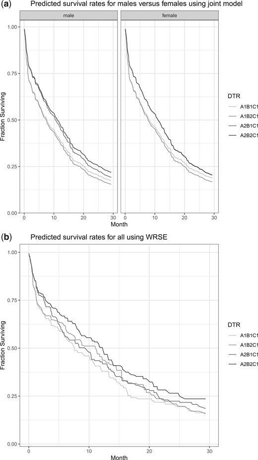
(a) The predicted survival probabilities of four dynamic treatment regimens (DTRs) stratified by sex using the proposed joint stage model from CALGB 8923 data. (b) The predicted survival probabilities of four dynamic treatment regimens (DTRs) for all patients using the weighted risk set estimator (WRSE) from CALGB 8923 data.
6. Discussion
We proposed a joint modeling framework to evaluate DTRs that include tailored sequences of treatments resulting from a SMART. Many previously proposed methods for data from a SMART with survival outcomes employ inverse probability weights and either treat survival time as a continuous outcome or compare survival rates between DTRs using non-parametric estimators. Our proposed model is based on Cox models with flexible non-parametric baseline hazards for time-to-response and time on second-line treatment. We demonstrated that our model provides equally unbiased survival estimates as the non-parametric methods, while offering many other advantages.
Compared to the non-parametric estimators, our model offers the following features: (i) adjusts for auxiliary covariates that includes not only baseline information but also potentially new covariates at the end of first-line treatment, (ii) has a mechanism to parameterize/measure each treatment’s effect within the DTR, their interactions, and interactions with auxiliary covariates (without assumptions of these effects within or between DTRs), (iii) easy adaptation between different SMART designs by setting certain |$\beta$|’s to 0, and (iv) the ability to estimate conditional survival functions conditioning on not only the particular DTR of interest, but also on what has been observed so far (e.g. |$\hat{S}(t \mid \text{response at }s)$| or |$\hat{S}(t \mid \text{no response by }s)$|).
The limitation of our model is that the non-parametric estimation of baseline hazards requires larger sample sizes (depending on the total number of unique time points from all subjects in the data) and longer computational time compared to other models where a distribution is assumed. In the setting of small samples, we can fit our model assuming some parametric distributions for the baseline hazards (e.g. Weibull). This will decrease the number of parameters needed to be estimated, yet still offers all of the advantages discussed.
Extension of the method can be made in a few directions. First, the proposed model has common covariates for time-to-response and time-to-death. This assumes that their dependence can be explained by the observed covariates. Further extension to this model such as inclusion of a common latent frailty term can be done to account for the unmeasured association between these two time-to-events. Second, the current model allows for new covariates that are available at second-line treatment initiation. Other time-dependent covariates can also be incorporated. Third, DTRs may have more than two stages (e.g. oncology trials) where multiple line of salvage therapies are available. The joint modeling approach has been implemented for 3 stages, so an analogous extension in the SMART setting is feasible.
The issue of multiple comparisons had not yet been fully addressed for survival data in the SMART setting. This may, in part, be due to the limited number of SMARTs having a survival endpoint that have been conducted and the lack of open access data for those that have. SMART designs with survival endpoints may be particularly challenging to implement based on requiring multiple drug treatments, an intermediate tailoring variable, and the time required to provide a sequence of treatments and monitor the time to event. Moreover, clinical collaborators may not fully understand the concept of DTRs and worry about multiple comparison issues in SMART design. It is especially important to motivate SMART design by interest in DTRs and to clearly communicate the definition of a DTR to clinical collaborators. Specifically, to clarify that each DTR includes two pathways in the SMART design, so that interest is not in the estimation and comparison of each individual treatment pathway, but rather in combinations of pathways which allow for more powerful and clinically meaningful comparisons. In order to identify the optimal DTR(s), SMARTs with many embedded DTRs may still require a large number of comparisons resulting in a loss of statistical power. We, therefore, adapted the previously proposed approach using multiple comparisons with the best for continuous outcomes to compare DTRs with survival outcomes which could help address clinical collaborators’ worries about multiple comparisons and facilitate a discussion on identifying the best DTR to inform clinical practice. We compared each DTR’s predicted survival rate at time |$t$| with the best of others and identified a set of DTRs that contains the true best DTR with a certain type I error rate. We outlined the procedure to find rejection rule that would satisfy such type I error and demonstrated the method with simulations. We are interested in developing a similar multiple comparison method to find the set of DTRs with the best survival across time (i.e. not just at time |$t$|), using restricted mean survival, for example. While we cannot address many of the barriers to implement a SMART design with a survival outcome, we hope that the development and dissemination of methods to analyze DTRs like those in this article will bolster the use of SMART design, inform clinical practice, and provide SMART data for future researchers.
Software
R code to simulate a SMART design II with survival outcomes, fit the joint model, and compare against previous methods is available from the GitHub at https://github.com/ycchao/code_Joint_model_SMART.
Supplementary material
Supplementary materials are available online at http://biostatistics.oxfordjournals.org.
Acknowledgments
Conflict of Interest: None declared.
Funding
Cancer Intervention and Surveillance Modeling Network (CISNET) (U01 CA199338); and University of Michigan Prostate Specialized Program of Research Excellence (SPORE) (P50 CA186786), both from the National Institute of Health/National Cancer Institute.
References
Author notes
Yan-Cheng Chao and Qui Tran authors contributed equally to this work.
