Modeling continuous glucose monitoring (CGM) data during sleep Free

Summary

1. Introduction

Diabetes is a chronic disease resulting from the pancreatic inability to produce insulin in reaction to blood glucose levels. There are two main types of diabetes. Type 1 diabetes is characterized by absolute insulin deficiency, whereas Type 2 is characterized by insulin resistance (WHO, 2016). In 2014, approximately |$422$| million people worldwide were living with Type 1 or 2 diabetes (WHO, 2016), with |$30$| million people being affected in the US alone (CDC, 2020). High levels of blood glucose observed in diabetes lead to increased risk of adverse health effects including retinopathy (Chen and others, 2011), cardiovascular disease (ERFC, 2010), lower extremity amputations (Moxey and others, 2011), cognitive dysfunction (Kodl and Seaquist, 2008), and premature morbidity and mortality (Zimmet and others, 2001). In this article, we focus on Type 2 diabetes, which constitutes |$90$|% of all cases (Zimmet and others, 2001) and “is tied to rising rates of overweight and obesity in adults as well as in youth” (Chen and others, 2011).

Diabetes diagnosis and management is traditionally based on measurements of the glycated hemoglobin HbA|$_{1c}$| (Selvin and others, 2010) in the blood. HbA|$_{1c}$| is associated with the average blood glucose over the preceding 8–|$12$| weeks (Nathan and others, 2007), and can be viewed as a summary of the long-term blood glucose profile. A normal glucose profile is non-constant, with typical normal values varying between |$70$| mg/dL and |$120$| mg/dL, with a “modest degree of variation” and characteristic spikes associated with meal intakes; see, for example, Figure 1 in Service (2013). The highly non-linear and non-stationary nature of normal glucose profiles is due to a wide range of environmental factors including time, quantity and composition of meals, physical activity time, intensity and type, stress, and sleep quality (ADA, 2004; Service, 2013).

Continuous glucose monitors (CGM) are small wearable devices that measure the glucose levels continuously throughout the day, with some monitors taking measurements as often as every 5 min (Rodbard, 2016). Data from these monitors provide a detailed quantification of the variation in blood glucose levels during the course of the day. However, while CGMs measure the time-dynamic of glucose profile and play an increasing role in clinical practice (Carlson and others, 2017), their measurements are highly dependent on environmental and behavioral factors (i.e., meals, physical activity) that are often unknown in observational studies.

Here, we analyze CGM profiles of study participants with Type 2 diabetes during time periods corresponding to actigraphy-estimated sleep. In contrast to day times, these periods are expected to be much less confounded by meals and physical activity. Recent evidence suggests that the blood glucose dynamics during sleep has an effect on the overall quality of glycemic control as measured by HbA|$_{1c}$| (Monnier and others, 2013). It has also been suggested that the rise in glucose values towards the end of the sleep period in the absence of a meal may lead to sleep hyperglycemia and impaired fasting glucose levels (Porcellati and others, 2013). However, these results were based on crude summaries of sleep-related CGM data (Monnier and others, 2013).

Our goal is to quantify the subject-specific blood glucose profiles during actigraphy-estimated sleep periods and investigate the association between these characteristics and levels of HbA|$_{1c}$|⁠. We propose a multilevel functional Beta model to characterize within- and between-subject variability and capture the highly heterogeneous nature of blood glucose profiles across study participants. The proposed model allows to construct subject-specific quantile bands for blood glucose profiles from sleep onset, which can be used to identify high-risk periods of sleep hypo- or hyperglycemia (Edelman and Blose, 2014) as well as study participants that may benefit from insulin administration to improve overall glucose control in future nights (Orszag and others, 2015).

2. Study description

2.1. Samples/study description

The study sample consisted of patients with Type 2 diabetes recruited from the general community. Eligibility criteria included having Type 2 diabetes with a glycosylated hemoglobin (HbA|$_{1c}$|⁠) value |$\geq$| 6.5% and not using insulin therapy. Individuals were screened with an overnight home sleep study using a type 3 sleep monitor. Only patients with an oxygen desaturation index |$\geq 15$| events/h were selected. After the initial screening procedures, eligible patients completed an actigraphy study using a Philips Actiwatch and continuous glucose monitoring using the Dexcom G4 sensor. The actigraph was worn on the non-dominant wrist and the Dexcom sensor was placed |$6$| cm lateral to the umbilicus. Participants were instructed to wear both monitors for |$7$| days and provide calibration glucose data for the Dexcom sensor twice a day as per manufacturer instructions. Informed consent was obtained from all study participants and the protocol was approved by the local Institutional Review Board of the Johns Hopkins University School of Medicine.

2.2. Data description and processing

For each study participant, sleep periods were estimated using the actigraphy data and the proprietary algorithm of the Phillips Actiwatch® wearable device. The actigraphy-estimated sleep periods were further analyzed to determine any missing periods defined as time gaps between consecutive sleep periods longer than |$36$| h. For study participants with at least three sleep periods available, these missing sleep periods were imputed using the estimated subject-specific median sleep duration and median wake-up time. This resulted in |$1307$| actigraphy-estimated sleep periods for |$124$| study participants ranging from |$4$| to |$15$| nights per study participant, with a median of |$11$| nights. These study participants have a median of 13 days of available CGM measurements (during both sleep and wake). The number of estimated sleep periods is smaller than the number of days of CGM measurements for some study participants as we only imputed missing sleep periods that occurred between two estimated sleep periods. Thus, no sleep periods were imputed before the first or after the last estimated sleep period using the Philips Actiwatch algorithm. The median estimated sleep duration across all study participants is 7 h with lower and upper quartiles of 6.3 and 7.5 h, respectively. We analyzed the first 7 h from estimated sleep onset (the results using the first 6 h were similar). Rather than stretching the shorter sleep trajectories to the same length (which may lead to distortion of circadian and sleep-related biological rhythms), we consider all sleep trajectories in absolute time from the actigraphy-estimated sleep onset, in accordance with established practices in physiological studies of glucose regulation during sleep in healthy subjects (Van Cauter and others, 1989, 1991).

While Dexcom G4 provides measurements of blood glucose levels every |$5$| min, the timings of these measurements are desynchronized across days and study participants. To address this problem, we linearly interpolated the BG trajectories to estimate glucose values at |$5$| min intervals from the estimated sleep onset (time zero).

2.3. Statistical challenges

Figure 1 displays the glucose trajectories during the first 7 h of actigraphy-estimated sleep for six study participants (selected to illustrate the variety of BG profiles observed in the data). Each black solid line corresponds to one period of actigraphy-estimated sleep and time |$0$| corresponds to the actigraphy-estimated sleep onset. The overall distribution of BG levels during the first 7 h of actigraphy-estimated sleep for all subjects in the study is provided in the Supplementary materials available at Biostatistics online.

Fig. 1.

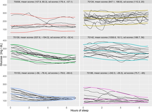
Glucose trajectories for six study participants during actigraphy-estimated sleep periods.

Open in new tabDownload slide

While not providing an exhaustive view of the entire data set, Figure 1 gives a good representation of the modeling challenges. First, each sleep period corresponds to a trajectory of BG levels, which leads to a multilevel functional structure (Di and others, 2009; Shou and others, 2015; Zipunnikov and others, 2011). Second, there are substantial differences within- and between-subjects both at the beginning and the end of the trajectory as well as in terms of the intra-night variability. Third, the within-subject marginal distributions (distributions of BG at a particular time across nights) are highly heterogeneous with some distributions being symmetric, while others exhibiting strong skewness and heavy tails. Fourth, the within-night trajectories can take a large number of potential shapes including increasing, decreasing, smooth, and highly variable patterns. Fifth, the beginning and end of the sleep period are estimated based on actigraphy measurements, and therefore are subject to measurement error. Finally, the data for some nights ends before the 7 h period, which leads to uneven domain functional data (Gellar and others, 2014; Johns and others, 2019).

2.4. Characteristics of a good model

Our goal is to introduce a flexible subject-specific model that estimates smoothly the marginal distributions of BG levels at each time point from the actigraphy-estimated sleep onset. Such a model should produce smooth means and marginal quantiles across time and should provide a good visual fit to the observed data. Another goal is to identify the main directions of variation and the relative importance of the characteristics of these distributions (e.g., time-dependent mean and variance). We propose to fit such a model by estimating the subject-specific marginal distributions using methods of moments, extracting their main directions of variation at the population level using functional principal component analysis (FPCA), and then use projections on these components for smoothing. This results in an estimator of the distribution of BG for each study participant at each time from the estimated sleep onset. Such an estimator could be used, for example, to check whether on a new night the BG level at a particular time is outside the subject-specific distribution, and thus identify high-risk profile deviations such as hypo- or hyperglycemia. It can also be used to provide baseline information for the amount of basal insulin administration to improve glucose control in future nights. Finally, the extracted subject-specific features of night glucose profile could be used to assess the effect of the blood glucose dynamics during sleep on study participants’ clinical characteristics, such as levels of hemoglobin HbA|$_{1c}$|⁠.

2.5. Limitations of existing functional multilevel models

While model (2.1) appears to be a natural choice for CGM data in our study, it does not capture important characteristics of the data; see Figure 1. First, the magnitude of the night to night variability differs across individuals, which could correspond to heteroscedasticity in the level 2 random effects ζ_ijl. Second, there is a strong correlation between the subject-specific mean and standard deviation processes (Section 4.2): the subjects with higher/lower average glucose values tend to have higher/lower variability, respectively. This violates the assumption of no correlation between Z_i(t) and W_ij(t) processes. Third, the KL expansions implicitly rely on the normality assumption for the within-subject marginal distribution of Y_ij(t). These issues lead to substantial difficulties in interpreting the results of mfPCA model (2.1) in this context. More details on the limitations of mfPCA model are provided in Supplementary materials A available at Biostatistics online.

3. A multilevel Beta model for CGM data

To address the specific observed structure of the CGM data, we propose to model the within-subject marginal distribution of |$Y_{ij}(t)$| using the four parameter Beta distribution. This allows modeling data with both negative and positive skew and accounts for the biological restrictions on the range of glucose values. For example, values below 40 mg/dL lead to the loss of consciousness, seizures and eventual death. We propose the marginal model |$Y_{ij}(t) \sim \texttt{Beta}\{\mu_i(t), \sigma_i(t), m_i, M_i\}$|⁠, where |$[m_i, M_i]$| is the support of the distribution, |$\mu_i(t)$| is the marginal subject-specific mean, and |$\sigma_i(t)$| is the marginal subject-specific standard deviation at time |$t$| after the actigraphy-estimated sleep onset. The standard parameterization of Beta distribution in terms of |$\alpha_i(t)$| and |$\beta_i(t)$| can be obtained using identities |$\mu_i(t) = \mathbb{E}\{Y_{ij}(t)\}=(M_i-m_i)\alpha_i(t)/\{\alpha_i(t)+\beta_i(t)\} + m_i$| and |$\sigma^2_{i}(t) = {\rm Var}\{Y_{ij}(t)\}=(M_i-m_i)^2\alpha_i(t)\beta_i(t)/\{\alpha_i(t)+\beta_i(t)\}^2\{\alpha_i(t)+\beta_i(t)+1\}$|⁠, where expectations are conditional on the subject. In this article, we work directly with mean and standard deviation parameterization. Both |$\mu_i(t)$| and |$\sigma_{i}(t)$| are allowed to vary with time and are assumed to be smooth functions. The model estimation procedure can be divided into a number of simple steps.

There exist several methods for FPCA (Yao and others, 2003; Ramsay and Silverman, 2005; Goldsmith and others, 2013), and we found that results were robust to the choice of the method (Supplementary Materials  Section B available at Biostatistics online). Here, we use FPCA via FACE (Xiao and others, 2016). In (3.2), |$\widehat \mu(t)$| is the estimated overall mean, which we obtain via cubic spline smoothing of |$\widetilde{\mu}(t)=I^{-1}\sum_{i=1}^I\widetilde \mu_i(t)$|⁠. Here, |$I$| is the total number of study participants, |$\widehat{\phi}_k(\cdot)$| are estimated eigenfunctions, |$\widehat{\xi}_{ik}$| are the estimated scores. The number of eigenfunctions, |$K$|⁠, is chosen to explain a certain percent of variance; see Xiao and others (2016) for more details on FACE implementation. We apply a similar procedure to obtain the smooth estimator |$\widehat \sigma_i(t)$|⁠. We start with the pointwise estimator of BG standard deviation, |$\widetilde{\sigma}_{i}(t)$|⁠, for study participant |$i$| at time |$t$|⁠, where |$ \widetilde{\sigma}^2_{i}(t) = \sum_{j=1}^{n_i(t)}\{Y_{ij}(t) - \widehat{\mu}_i(t)\}^2/\{n_i(t) - 1\}\;. $| The standard deviation estimators based on |$\widetilde{\mu}_i(t)$| instead of |$\widehat{\mu}_i(t)$| are similar, but slightly smaller. We obtain smooth |$\widehat \sigma_i(t)$| from |$\widetilde \sigma_i(t)$| via truncated FPCA as above.

We propose to evaluate the subject-specific support |$[m_i, M_i]$| based on the observed range of all (day and night) BG values for each individual. This is reasonable as Riddlesworth and others (2018) reported that 10–14 days of CGM data are sufficient to provide good estimation of CGM metrics, and in our study 75% of the study participants had at least 10 days of CGM measurements (median 13 days). Inclusion of both wake and sleep periods in the estimation of |$[m_i, M_i]$| also avoids potential problems due to measurement errors in sleep period estimation.

Once the beta parameters are estimated, the pointwise quantiles for |$Y_{ij}(t)$| are estimated by |$q_{\alpha,Y}=m_i+(M_i-m_i)q_{\alpha,Z}$|⁠, where |$q_{\alpha,Z}$| is the |$\alpha$|-quantile of the corresponding Beta distribution.

4. Results

We apply the model described in Section 3 to the blood glucose data from Section 2. In Section 4.1, we describe the estimation of smooth subject-specific means |$\mu_i(t)$| and standard deviations |$\sigma_i(t)$|⁠. In Section 4.2, we investigate associations between the estimated FPCA scores and levels of hemoglobin HbA|$_{1c}$|⁠. In Section 4.3, we provide the distribution of subject-specific BG ranges. In Section 4.4, we illustrate the estimated point-wise quantiles for six selected subjects and assess goodness-of-fit via qqplots.

4.1. FPCA on subject-specific means and standard deviations

We first construct estimators of subject-specific means |$\widehat \mu_i(t)$| (3.2) based on the FACE algorithm (Xiao and others, 2016) as implemented in the R package refund (Goldsmith and others, 2019). The spline smoothing parameter is selected to minimize pooled generalized cross-validation criteria. We select the number of principal components |$K$| to explain 99% of variance leading to |$K=3$|⁠. We also considered smoothing covariance matrix via penalized splines (Di and others, 2009; Goldsmith and others, 2013) as implemented in function fpca.sc within the same package, but results were similar. While by default FACE uses 35 knots, we only used 5 knots because: (i) the length of the time grid |$T=84$| was quite short; (ii) the FACE eigenfunctions with 5 knots are visually smoother and more interpretable than those obtained using 35 knots; (c) the overall shape of the estimated FACE eigenfunctions with 5 knots and 35 knots are almost identical. Since the number of sleep trajectories varies from 4 to 15 across study participants, we also implemented a weighted FPCA, but results were identical to unweighted FPCA. Using subsampling of study participants, we showed the robustness of the estimated means and eigenfunctions, indicating that the varying number of curves has little effect on estimation; see details in Supplementary Materials  Section C.

The left panel in Figure 2 displays the initial pointwise estimators of the BG means, |$\widetilde{\mu}_i(t)$| (red lines), together with the smooth mean estimates, |$\widehat{\mu}_i(t)$| (blue lines), for the six study participants in Figure 1. The right panel in Figure 2 displays the estimated smooth means, |$\widehat{\mu}_{i}(t)$|⁠, for all |$124$| study participants with the same six study participants highlighted in blue. Results indicate that mean estimation is quite reasonable.

Fig. 2.

Left: Pointwise means |$\widetilde \mu_i(t)$| (red) versus fPCA smoothed means |$\widehat \mu_i(t)$|(blue) for six selected study participants. Right: Smoothed subject-specific means |$\widehat \mu_i(t)$| for all |$124$| study participants, the |$6$| participants from Figure 1 are highlighted in blue. This figure appears in color in the electronic version of this article, and color refers to that version.

Open in new tabDownload slide

We similarly construct smooth estimators of subject-specific standard deviations based on truncated FPCA of |$\widetilde \sigma_i(t)$|⁠. While |$K=6$| components are needed to explain 99% of variability, we used |$K=3$| components because: (i) they explain 93% of variability; (ii) each of the last 3 component contributed less than 2% of variability; and (iii) |$K=6$| components led to overfit of standard deviation processes for subjects with outlying trajectories; see Supplementary Materials  Section C available at Biostatistics online for more details.

Figure 3 displays the overall mean and principal components for the subject-specific mean (top three panels) and standard deviation processes (bottom three panels). The overall (population) BG mean, |$\widehat{\mu}(t)$|⁠, shown in the top left panel indicates a continuous, linear decrease in average BG levels for the first |$6$| h. The mean decreases from around |$165$| mg/dL to around |$137$| mg/dL, or |$17$|%, from estimated sleep onset. After hour |$5.5$|⁠, the overall mean levels off. The mean standard deviation function follows a similar pattern decreasing roughly linearly from around |$35$| mg/dL to around |$15$| mg/dL, or more than |$50$|% in the first 7 h from the actigraphy-estimated sleep onset. This is due, at least in part, to the funnel effect of the data in some of the study participants (e.g., study participants 70139, 70153, and 70186 shown in Figure 1).

Fig. 3.

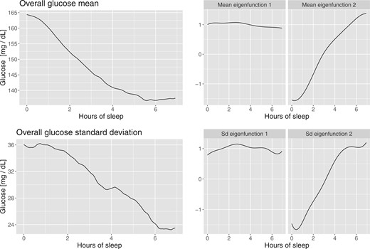
Functional PCA applied to point-wise means and standard deviations of glucose values.

Open in new tabDownload slide

The first two principal components of the subject-specific mean processes are shown in the top middle and right panels of Figure 3. After smoothing these two principal components explain |$98$|% of the variability. The first principal component is a shift in mean, while the second is close to a linear trend. This indicates that using the first two principal components is roughly similar to using a random slope random intercept mixed effects model for the mean processes. The first two principal components for the standard deviation processes look remarkably similar to those of the mean and explain 90% of the variability after smoothing. Again, this indicates that a random intercept random slope model could be appropriate for the standard deviation processes.

4.2. Interpretation of estimated scores from FPCA

For interpretation purposes, recall that the first two principal components for the mean processes correspond to the subject-specific mean and rate of decrease in the mean BG levels, respectively. The first two principal components for the standard deviation processes correspond to the subject-specific standard deviation and rate of decrease in standard deviation of BG levels, respectively.

Figure 4 displays the scores for the principal components of the mean and standard deviation processes. The first panel corresponds to the first principal component scores of the mean (x-axis) and standard deviation (y-axis) processes. The high positive correlation between these scores (⁠|$\rho=0.61$|⁠) indicates that study participants who have higher average BG levels tend to have higher variability. The second panel corresponds to the second principal component scores of the mean (x-axis) and standard deviation (y-axis) processes. The moderate positive correlation (⁠|$\rho=0.47$|⁠) between these scores indicates that study participants whose mean decreases tend to have a standard deviation that also decreases over the course of the night.

Fig. 4.

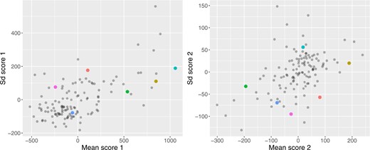
Association between mean and standard deviation scores from the functional PCA, the colored dots correspond to the six selected study participants. This figure appears in color in the electronic version of this article, and color refers to that version.

Open in new tabDownload slide

Figure 5 displays the scores of the subject-specific mean (left panel, x-axis) and standard deviation (right panel, x-axis) on their first principal components versus HbA|$_{1c}$| (both panels, y-axis). Both associations are linear with correlations of |$0.79$| for the mean scores and HbA|$_{1c}$|⁠, and |$0.6$| for the standard deviation scores and HbA|$_{1c}$|⁠. The correlation with the other scores is less than |$0.21$|⁠. Using a linear model to predict HbA|$_{1c}$| with all the scores (⁠|$3$| for mean and |$3$| for standard deviation) indicates that the scores of the mean process on the first and second principal components, and the score of the standard deviation on the first principal component are significant. The |$R^2$| value for a model including these three scores is |$0.70$| compared to an R|$^2$| of |$0.64$| if we include only the scores on the first principal components of the mean and standard deviation processes. These results indicate that HbA|$_{1c}$| is associated both with the mean and standard deviation of BG levels, as well as with the rate of change of BG after the actigraphy-estimated sleep onset. This does not mean that the other scores are not important, just that they are less important for quantifying the association with HbA|$_{1c}$|⁠. In fact, it could very well be that the observed variability in the other components may be associated with health outcomes or other biomarkers. At the very least, we provide a simple decomposition of marginal mean and standard deviation processes of BG processes after actigraphy-estimated sleep onset.

Fig. 5.

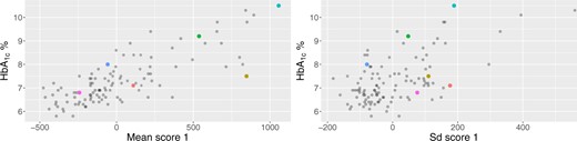
HbA|$_{1\mbox{c}}$| (y-axis) versus scores on the first principal components of the subject-specific mean (x-axis, left panel) and standard deviation (x-axis, right panel) processes. The colored dots correspond to the |$6$| selected study participants. This figure appears in color in the electronic version of this article, and color refers to that version.

Open in new tabDownload slide

Given that both HbA|$_{1c}$| and continuous glucose monitors (CGMs) provide estimates of the same target, long-term average blood glucose, one could ask why the correlation is not stronger. Here, we identify three potential explanations. First, we focused only on the first 7 h from the actigraphy-estimated sleep onset rather than the entire |$24$| h time period. Second, we have an average of only |$\sim$|10.5 actigraphy-estimated sleep periods per study participant, whereas HbA|$_{1c}$| targets the mean over the previous 2–|$3$| months. Third, it is likely that HbA|$_{1c}$| is a weighted average of BG, where the weights may be unknown, depend on the individual and larger for more recent days.

4.3. Distribution of BG level ranges

Figure 6 displays the subject-specific range of BG values, |$[m_i, M_i]$|⁠, where the study participants are sorted from the minimal to the maximal value of |$M_i$|⁠. As discussed in Section 3, both |$m_i$|⁠, |$M_i$| are estimated over all time points (including both sleep and wake periods). There are several potential problems with this approach including: (i) the minimum and maximum values depend on the number of data points available; (ii) minimum and maximum are sensitive to noise; and (iii) interpretation may be difficult given the dependence on time. One alternative is to consider the model with the same conservative range |$[m, M]$| for all subjects with |$m=\min m_i$| and |$M=\max M_i$|⁠. We do not pursue this approach here since BG ranges exhibit high variability across subjects (Figure 6). Allowing for such a wide support of the Beta distribution forces a symmetric distribution for individuals with tighter glucose control but highly skewed distributions. Moreover, because |$m_i$| and |$M_i$| are based on both sleep and wake periods, the corresponding values are unaffected by possible errors in actigraphy-based estimation of sleep times and the non-wear periods of actigraphy device. More details on the calculation of |$m_i$| and |$M_i$| are provided in the Supplementary materials B available at Biostatistics online. We evaluated the sensitivity of estimated quantiles to misspecification of |$m_i$| and |$M_i$|⁠, and found that the approach still performs well under mild and reasonable deviations; see Section 4.5.

Fig. 6.

Minimum and maximum glucose values |$[m_i, M_i]$| for |$124$| study participants from the study sorted by |$M_i$|⁠, the maximal observed value of BG over all days and times.

Open in new tabDownload slide

4.4. Model fit for individual study participants

As we described in Section 3, the fitted multilevel Beta model provides estimates of the subject-specific marginal quantiles of the BG distributions. We assess the fit of corresponding model by examining QQ plots at a global (all subjects and times), time-specific (all subjects for a given time), and subject-specific (all times for a given subject) levels. For each subject |$i$| and time |$t$| from actigraphy-estimated sleep onset, we plot the sorted glucose values |$Y_{ij}(t)$|⁠, |$j=1, \dots, n_i(t)$|⁠, versus the theoretical quantiles of the fitted Beta distribution corresponding to |$0.5/n_i(t), \dots, 1 - 0.5/n_i(t)$| percentiles. We then overlay these plots over both subjects and times (global), over subjects for a given time |$t$| (time-specific), and over times for a given subject |$i$| (subject-specific). Figure 7 displays the corresponding global QQ plots for the Beta marginal distribution, time-specific QQ plots for |$t\in\{1, 2\}$| hours from sleep onset, and subject-specific QQ plots for two selected subjects in the study. For reference, we also consider QQ plots based on marginal Normal distribution with mean |$\widehat \mu_i(t)$| and standard deviation |$\widehat \sigma_i(t)$| obtained as described in Section 3. The QQ plots indicate that the Beta model results in unbiased quantile estimation. In contrast, the normal-based model leads to substantial bias at lower quantiles. Indeed, the left panels in Figure 7 indicate that the Normal model (red dots) tends to substantially underestimate the lower quantiles (see box in the left-bottom corners of the two panels) relative to the Beta model (blue dots). This is likely due to symmetric form of the Normal distribution combined with its unbounded support. The bias induced by Normal models is more pronounced at lower values of |$t$| for individuals with highly skewed distributions, such as 70186. In individuals with more symmetric data (e.g., study participant 70142), the Beta and the Normal model give similar results, whereas in skewed cases (study participant 70186) the Beta model estimates the quantiles much better.

Fig. 7.

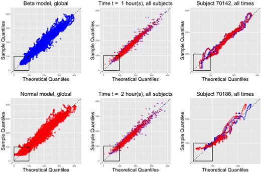
QQ plots based on theoretical Beta (blue circles) or Normal (red triangles) distributions based on all subjects and times (1st column), all subjects for two selected times (2nd column), and all times for two selected subjects (3rd column). The Normal distribution tends to be biased at lower quantiles, which is likely due to its unbounded support. This bias tends to be more prominent at lower values of |$t$|⁠, and for subjects with skewed distributions (70186). For subjects with symmetric distributions (70142), the difference between Beta and Normal model fits is less pronounced.

Open in new tabDownload slide

Figure 1 displays the corresponding fitted median, 2.5% and 97.5% pointwise quantiles for the six study participants using the Beta distribution. While most study participants have quantiles that are roughly symmetric around the median, they are not for study participant 70186. Visually, the quantile estimates look reasonable for four out of the six study participants (⁠|$70134$|⁠, |$70142$|⁠, |$70153$|⁠, and |$70186$|⁠). The estimated |$2.5$| quantile for study participant |$70056$| is substantially lower than where one would it expect it given the observed data. This effect is likely due to the extreme positive skewness and the small number of actigraphy-estimated sleep periods for this individual. In contrast, the estimated |$97.5$| quantile for study participant |$70139$| seems to be larger than what one would expect from a visual inspection of the data. This is likely due to the strong negative skew in the data; note the higher density of curves at higher level of BG.

The colors used for median and quantile estimators in Figure 1 are subject-specific and correspond to the colors of the dots in Figures 4 and 5, respectively. This provides an additional layer of interpretation for the results. Consider study participant 70142 (shown in cyan), which appears in the extreme right side of the left panel of Figure 4. This indicates both a relatively high mean and standard deviation BG, which confirms the visual inspection of the BG traces. The same study participant in the right panel of Figure 4 has a score close to zero on the second principal component of the mean process (linear trend) indicating a slow decrease in the mean BG from the actigraphy-estimated sleep onset. The score on the second principal component of the standard deviation process (linear trend) is positive and large, which corresponds to no decrease or slight increase in the standard deviation process from the actigraphy-estimated sleep onset. In contrast, study participant 70153 (shown in blue) is almost at the opposite end of the plot in both panels of Figure 4. The reason for this contrast in the left panel of Figure 4 is that the study participant 70153 (shown in blue) has a lower BG mean (hence a smaller score on the first principal component of the mean) and a lower BG standard deviation (hence a smaller score on the first principal component of the mean). The reason for this contrast in the right panel of Figure 4 is that this study participant has a BG mean that decreases more rapidly (hence a smaller score on the second principal component of the mean) and a BG standard deviation that decreases more rapidly (hence a smaller score on the second principal component of the mean) compared to participant 70142 (shown in cyan). From Figure 1, the BG trajectories of the study participant coded in blue are lower, closer, and have a more pronounced funnel effect than those of the study participant coded in cyan.

We now investigate the same two study participants in the two panels of Figure 5. The study participant shown in cyan has the largest HbA|$_{1c}$| in our study at |$10.5$|% and the highest score on the first principal component of the mean process. For this reason, the corresponding cyan point appears in the extreme upper corner of the left panel of Figure 5. The study participant shown in blue has a large HbA|$_{1c}$| in our study at |$8$|%, though the score on the first principal component is not that large, which, corresponds, indeed, to a much lower mean BG from the actigraphy-estimated sleep onset. The right panel of Figure 5 completes the picture, indicating that the study participant shown in cyan also is among the top five study participants in terms of standard deviation of BG trajectories from actigraphy-estimated sleep onset. In contrast, the study participant shown in blue is at the other end of the spectrum in terms of standard deviation. These findings are highly consistent with the visual inspection of the data but have the added benefit that they quantify these observations. We posit that identifying study participants, such as the ones shown in cyan and blue, who both have large HbA|$_{1c}$| but completely different BG dynamics after actigraphy-estimated sleep onset could suggest further, more focused study of these individuals and potentially more targeted interventions or therapies.

Some of model fits in Figure 1 could be viewed as disappointing, at least for some of the study participants (e.g., the |$2.5$| quantile of the study participant 70058). However, these imperfections underline the complexity of the problem, even when we simplified it to achievable goals. The main problem is that approximately |$15$|% of study participants exhibit either positive or negative skew in their sleep profiles. Thus, a data transformation such as the log or square root would tend to reduce the problem for the positively skewed distributions, but exacerbate it for negatively skewed distributions. Another alternative would be to use subject-specific transformations or distributions. For example, the log transformation works well for positively skewed distributions, but not for those with low or negative skew. However, what ones gain in fit one loses in interpretation of simple quantities, such as the mean or standard deviation when different transformations are applied across study participants. Additional comparisons of quantile estimation methods are provided in Supplementary materials D available at Biostatistics online.

4.5. Assessment of quantile estimation under support misspecification

Supplementary materials F available at Biostatistics online display corresponding percent difference values for the perturbed Beta and Normal distribution for all values of |$p\in[0.01,0.99]$|⁠.

On average, the 5% perturbation of support leads to at most 1% change in quantiles which is most pronounced at the lower tail (with the average difference |$\widetilde d(p) < 0.5\%$| for |$p \in (0.05, 0.98)$|⁠). As expected, the maximal difference |$d_{\max}(p)$| is larger, however is always below 7% and only 4% on average. Thus, the estimated quantiles under the Beta model are robust to some misspecification in the minimal and maximal values.

In contrast, using the Normal distribution with unbounded support leads to large differences in the lower tails (⁠|$d^{\text{norm}}(p) > 5\%$| for |$p \in (0.01, 0.05)$| and |$d^{\text{norm}}_{\max}(p) > 20\%$| for |$p\in (0.01, 0.2)$|⁠). This is likely due to the pronounced right skew of the marginal subject-specific distributions for many study participants; see Figure 2. This reinforces the results reported in the lower left corners of the QQ plots of Figure 7.

For the second sensitivity analysis, we generate synthetic CGM data with pre-specified marginal subject-specific distributions (either Normal or Beta), and misspecify |$m_i$| and |$M_i$| values by an average of 20 mg/dL. We simulate |$n=124$| subjects, each with |$n_j=14$| sleep periods. The data-generating mechanism produces synthetic data that closely mimics the real CGM data; see Supplementary materials E available at Biostatistics online. While the differences between the Normal and Beta models are hard to delineate visually, these differences are clear when we simulate a larger number of curves per study participant. Inspection of these plots indicate that the Beta distribution leads to more realistic synthetic data as it: (i) allows to generate skewed data and (ii) generates curves in the biological range of blood glucose, whereas the Normal model can easily generate unrealistic values. The data-generating process is described in the Supplementary materials E available at Biostatistics online.

Let |$F_{it}$| be the true marginal distribution of glucose values for subject |$i$| at time |$t$|⁠, and let |$q_{\alpha, it}$| be the corresponding |$\alpha$|-quantile. Let |$\widehat q_{\alpha, it}^{\mbox{normal}}$| and |$\widehat q_{\alpha, it}^{\mbox{beta}}$| be the estimated |$\alpha$|-quantiles for subject |$i$| at time |$t$| using multilevel functional Normal and Beta model (with misspecified support), respectively. To evaluate the quantile estimation performance, we calculate the quantile differences |$q_{\alpha, it} - \widehat q_{\alpha, it}^{\mbox{normal}}$| and |$q_{\alpha, it} - \widehat q_{\alpha, it}^{\mbox{beta}}$| for |$\alpha\in \{0.05, 0.1\}$|⁠. We focus on the lower quantiles as they typically correspond to glucose values near hypoglycemia range, a dangerous condition of low blood sugar that may lead to loss of consciousness, seizures and, in the extreme cases, death.

Supplementary materials F available at Biostatistics online contain boxplots of the quantile differences across both models and data-generating distributions. Not surprisingly, the best performance is achieved when the model matches the underlying data distribution. When the true data-generating distribution is Normal, the Beta model typically provides unbiased estimation of quantiles, with slight upward bias for the |$5$|% quantile (median difference of 2 mg/dL with IQR of 3 mg/dL). In some cases, the true quantile value is below 40 mg/dL, the minimal value of glucose observed across all study participants in the study and a borderline value for severe hypoglycemia. This result reinforces the idea that the Normal model can provide implausible small values of the glucose. When the true data-generating distribution is Beta, we consider separately |$23$| study participants with strong positive skew (average skewness across all times larger than |$0.6$|⁠). For the |$10$|% quantile, the Normal model leads to unbiased estimates for study participants with low to moderate skewness, and slight downward bias for participants with strong skew (median difference of |$-$|3 mg/dL with IQR of 4 mg/dL). The bias for |$5\%$| quantile is larger, especially for study participants with higher positive skew (median difference |$-$|9 mg/dL with IQR of 8 mg/dL). This bias could have important practical consequences if the estimated quantiles are used for management of BG. While the slight upward bias in the lower quantiles may lead to more false positive alerts of high blood glucose, the downward bias can be more dangerous. Indeed, this could lead to individuals not being alerted when their glucose levels are low, which is especially dangerous during sleep. In the real CGM data, the lower estimated quantiles for the Beta model either coincide or are higher than the Normal model quantiles. In summary, even when the underlying true distribution is symmetric and has unbounded support, there is a very high level of agreement with quantiles estimated using Beta distribution with bounded support. When the true distribution is skewed and the support is bounded, the Beta model performs well even with misspecified support.

5. Discussion

In this article, we focused on modeling CGM measurements of BG during periods of actigraphy-estimated sleep. We chose these periods because the confounding effects of activity and meals are expected to be smaller compared to the day period. A limitation of this approach is that the analyzed BG trajectories are not representative of the long-term BG average. Instead, we characterized the directions of variation of the within-subject means and standard deviations (across nights) at all time points from actigraphy-estimated sleep onset. Results indicate that: (i) both the mean and standard deviation processes can reasonably be captured by two principal components, one for the shift in mean and one for a linear trend; (ii) the scores on some of these components (first principal components of the mean and standard deviation) are strongly associated with HbA|$_{1c}$|⁠, the current standard for assessing the severity of diabetes; and (iii) there are clear differences in mean and standard deviation processes among study participants, which may provide additional information for personalized therapies.

The multilevel functional Beta model can produce estimators of the marginal quantiles at every time point from the actigraphy-estimated sleep onset. The estimated quantile bands could potentially be used for the management of BG during future nights. For example, some of the study participants have extremely high levels of HbA|$_{1c}$| (⁠|$>$|9 %) coupled with consistently high BG levels during the night (⁠|$>$|180 mg/dL), and thus these individuals may benefit from more targeted clinical and behavioral interventions. The achieved characterization of the subject-specific night profiles provides a useful baseline for the mean and variability of night glucose profiles, and could identify individuals who will most benefit from additional insulin administration and have the lowest risk of night hypoglycemia. Thus, re-analyzing the BG profiles after intervention (e.g., insulin administration or behavioral changes) could provide quantification of the intervention effect both at the individual and group levels.

The model proposed has several limitations that provide opportunities for further methodological and scientific research. For example, the estimands in the model are the marginal distributions at every time point from actigraphy-estimated sleep onset. This model was not designed to and does not capture the individual trajectories or cannot be used for dynamic prediction. For example, given a specific night’s BG history up to a particular point (say, |$2$| h after actigraphy-estimated sleep onset) and the BG trajectories over previous nights, one could be interested in providing a prediction and confidence intervals for BG levels at future points (e.g, |$3$| and |$4$| h after sleep onset). Such dynamic prediction could be used to identify periods of extreme hypo- and hyper-glycemia that may be particularly dangerous for the study participant. Our current model is not designed to do that.

Another limitation is that the model does not seem to fit all marginal quantiles in accordance to what would be reasonable from a visual inspection of both individual subject profiles and QQ plots. However, the multilevel Beta functional model seems to provide a better balance than simpler models already published in the literature (e.g., multilevel PCA). When used as a starting point for simulating synthetic data, it seems to provide more realistic datasets, especially when data are strongly skewed.

Our model quantifies the between- and within-subject BG variability during sleep based only on BG measurements during sleep. It is possible to improve the model by taking into account some characteristics of BG profile before the estimated sleep onset. For example, the BG levels in the first hours from estimated sleep onset are likely affected by the time since last meal and the last meal’s composition (e.g., carbohydrate and sugar content). Unfortunately, neither exact meal times nor meals’ composition are known in our study. Based on the visual inspection of 24-h subject’s profiles (see Supplementary materials available at Biostatistics online), it may be possible to identify meal times for some subjects based on the observed “hills.” However, at this time, we do not have a gold standard validating that these features in the data are proxies for timing and composition of the meals. Moreover, these features cannot be reliably estimated for all individuals in our study and we leave this interesting investigation for future research.

Finally, our focus is on quantifying main directions of between-subject variation in mean, standard deviation, and quantile processes at a given time point from estimated sleep onset. Thus, we do not directly model the autocorrelation of BG profiles at the individual level. At least in theory we have a working hypothesis that the current model could be extended to account for these features by combining it with the functional copula model of Staicu and others (2012). This extension is not straightforward because it would need to take into account the multilevel structure of the data.

Software

A GitHub repository https://github.com/irinagain/cgm-multi-level-beta contains the R code used for the data analyses and creation of figures in the article, along with a simulated CGM data that mimics characteristics of the real CGM data analyzed in the article.

Supplementary material

Supplementary material is available online at http://biostatistics.oxfordjournals.org.

Acknowledgments

We thank the A.E. and two anonymous reviewers for helpful comments that helped significantly improve this manuscript.

Conflict of Interest: Dr. Crainiceanu is consulting for Bayer and Johnson and Johnson on methods development for wearable computing. The current research is not related to his consulting.

Funding

National Institutes of Health (NIH) (F32 HL083640, R01 HL075078, R01 HL117167, R01 HL123407, and R01 NS060910.)

References