


Summary
Multistate models provide a powerful framework for the analysis of life history processes when the goal is to characterize transition intensities, transition probabilities, state occupancy probabilities, and covariate effects thereon. Data on such processes are often only available at random visit times occurring over a finite period. We formulate a joint multistate model for the life history process, the recurrent visit process, and a random loss to follow-up time at which the visit process terminates. This joint model is helpful when discussing the independence conditions necessary to justify the use of standard likelihoods involving the life history model alone and provides a basis for analyses that accommodate dependence. We consider settings with disease-driven visits and routinely scheduled visits and develop likelihoods that accommodate partial information on the types of visits. Simulation studies suggest that suitably constructed joint models can yield consistent estimates of parameters of interest even under dependent visit processes, providing the models are correctly specified; identifiability and estimability issues are also discussed. An application is given to a cohort of individuals attending a rheumatology clinic where interest lies in progression of joint damage.
1. Introduction
Life history processes in which individuals experience certain events or pass through different stages are central to chronic disease, health services research, economics, the social sciences, and other areas. Information needed to model, understand, and manage such processes is typically obtained through a variety of sources including longitudinal surveys and cohort studies, observational data from registries or clinics, and administrative records. Such sources often provide data collected at specific times over some period, and give an incomplete picture of individuals’ life histories. Moreover, to make valid inferences from such data it is important to consider whether there is a relationship between the life history process of interest and the observation process. Two crucial aspects of observation are (i) censoring or termination of the observation period for an individual due to, for example, loss to follow-up and (ii) the repeated assessment times at which data are collected on individuals. Standard methods of life history analysis depend on independence and ignorability assumptions of the observation process (e.g. Farewell and others, 2017; Kalbfleisch and Prentice, 2002, Section 6.2; Aalen and others, 2008, Section 2.2.8; Cook and Lawless, 2014; Cook and Lawless, 2018). These assumptions are necessary for the analysis of event history processes (Andersen and others, 1993; Aalen and others, 2008), which we focus on here, as well as the analysis of discrete or continuous outcomes in longitudinal studies (Molenberghs and Fitzmaurice, 2009; Farewell and others, 2017).
Much work has been carried out on dropout in longitudinal studies in which responses are measured at scheduled assessment times (Robins and Rotnitzky, 1995; Little and Rubin, 2002). Censoring or loss to follow-up in studies of failure time processes has also received considerable attention with numerous authors proposing joint models in which failure and censoring times are dependent (e.g. Fisher and Kanarek, 1974; Slud and Rubinstein, 1983; Scharfstein and Robins, 2002; Siannis, 2011). Independence assumptions cannot be checked using only the observed (incomplete) data, and the primary use of these joint models has been to assess the sensitivity of inferences based on independence assumptions to violations of such assumptions. A few authors (e.g. Baker and others, 1993; Frangakis and Rubin, 2001; Farewell and others, 2003) have discussed how data obtained by tracing persons after they become lost to follow-up (LTF) can be used to check independent censoring assumptions or to estimate a failure time distribution in the presence of dependent censoring. Cook and Lawless (2018) review this area and propose some new approaches.
This article has been partially motivated by our experiences with cohort studies involving persons at the Centre for Prognosis Studies in Rheumatic Disease at the University of Toronto. In these studies, individuals registered in disease clinics have periodic scheduled visits. However, patients often miss scheduled visits, and the actual times they visit a clinic are often unequally spaced in time and differ across individuals. A key concern is that the timing of visits may be related to a person’s disease history. They may also become LTF and be declared so, when they have not visited the clinic for some long period. In the absence of a precise definition of a LTF time, the LTF “event” may be viewed, in some sense, as a conceptual phenomenon. However, we view it as real event by virtue of the fact that the individual is truly no longer under study; the fact that the corresponding LTF time is not observed for many (or all) individuals is a complication that can be dealt with. Later in the article, we consider an illustration involving the University of Toronto Psoriatic Arthritis Cohort (Gladman and Chandran, 2011), a registry of patients that was started in 1977 and which now has over 1800 members; in this setting patients do not typically report a withdrawal time and the study investigators cannot likewise specify a particular time of LTF other than through specification of a post hoc rule.
Our aim in this article is to study independence assumptions related to intermittent observation times for life history processes, which has received much less attention than loss to follow-up (Keiding, 2014, Section 7.2). Grüger and others (1991), Cook and Lawless (2007, Section 7.1), and Cook and Lawless (2018, Section 5.4) presented independence conditions for intermittent observation and discussed likelihood-based inferences for event history analysis. More recently, several authors have discussed processes governing intermittent observation times and conditional independence conditions, so as to facilitate the use of inverse-intensity-of-visit (IIV) weighted estimating functions (e.g. see Lin and others, 2004; Buzkova and Lumley, 2007, 2009; Buzkova, 2010; Pullenayegum and Feldman, 2013; Pullenayegum and Lim, 2016). Farewell and others (2017) considered related ignorability conditions for the analysis of general longitudinal data. Neuhaus and others (2018) and McCulloch and Neuhaus (2020) consider mixed generalized linear models and intermittent observation times for discrete or continuous longitudinal responses through shared random effects models. There has, however, been limited discussion of dependence and of ways to assess and handle it in life history analysis aside from the case of survival analysis (e.g. Betensky and Finkelstein, 2002; Lawless and Babineau, 2006).
This article has two main objectives: the first is to consider joint models for life history processes and processes governing intermittent observation to accommodate specific types of dependence and examination of independence assumptions. The modeling framework we employ was introduced by Lange and others (2015); we extend their treatment by specifying independence conditions, by considering estimability of dependence models, and by examining the effects of dependence in some important practical settings. The second objective is to consider types of supplementary information that allow independence assumptions to be assessed. We carry out this work in the context of multistate life history processes, which include as special cases failure time, competing risks, and recurrent event models (e.g. Andersen and others, 1993; Beyersmann and others, 2012; Willekens, 2014; Cook and Lawless, 2018). The joint modeling framework is based on extending the corresponding multistate models to include states depicting the cumulative number of observation times.
Section 2 discusses independence conditions, introduces joint multistate models for life history and intermittent observational processes, and describes estimation based on them. Section 3 discusses estimation for Markov processes, examines estimability issues, and presents numerical studies on the effects of dependent visit times on standard estimators as well as estimators from the joint model. Section 4 gives an application involving data from a psoriatic arthritis clinic. Section 5 considers types of supplementary data that can be used to assess independence, and Section 6 contains concluding remarks.
2. Multistate models and intermittent observation schemes
2.1. Conditionally independent observation schemes
We consider life history processes in which individuals occupy and move among a set of |$K$| states over time. We let |$\mathcal{S} = \{1, \ldots, K \}$| denote the state space and let |$Z(t)$| represent the state occupied by a generic individual at time |$t \ge 0$| since the origin of the process. We focus on continuous-time models for the process |$\{Z(t), t \ge 0 \}$| which may also involve fixed or external (Kalbfleisch and Prentice, 2002) time-varying covariates |$\{ X(t), t \ge 0 \},$| and we let |$H(t^-) = \{Z(s), X(s), 0 \le s < t \}$| denote the history of the states occupied, and covariates, up to time |$t^-$|. The multistate model can be specified in terms of the transition intensity functions
for |$k \neq l \in \mathcal{S}$| (Andersen and others, 1993). Figure 1 shows state-space diagrams for four processes that we will refer to later: (a) is a failure time model, (b) is an illness-death model, (c) is an alternating (reversible) two-state model, and (d) is a simple progressive model.
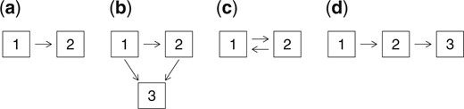
State-space diagrams for some multistate processes.
In some studies individuals may be effectively followed continuously, so that the times of all transitions from one state to another are recorded. This is the case when the transitions correspond to times of events that are readily apparent, such as a myocardial infarction, serious stroke, or death. The more common situation is that data on individuals are collected at intermittent observation times. This is the case in disease cohort studies, and so we refer to these occasions as visits and refer to the observation times as visit times. We focus here on this situation.
We now consider data from a single individual and let |$A_0$| denote the time of the first observation. If |$A_0 > 0,$| then the life history process has been active for some time prior to observation and in these cases baseline information on covariates and prior life history data are often available. We condition on |$A_0 = a_0$| and the observed life history information at |$a_0$| including |$Z(a_0)$| and proceed under the assumption that this is an independent delayed entry time (Keiding, 1992). We let |$E$| denote a defined (fixed) administrative end-of-follow-up time which may differ across individuals. In many settings an individual may be randomly LTF before |$E$|, and we let |$C < E$| represent a potential premature LTF time; in some settings |$C$| may be reported exactly and in other scenarios it may be unobserved, but the distinction between these two scenarios is not necessary provided the LTF time is conditionally independent given the observed process history. Data on an individual are collected at random visit times after the baseline assessment; we let |$m$| denote the realized number and let |$a_1 < a_2 < \cdots < a_m$| denote the realized visit times after the baseline assessment at |$a_0$|. Data |$D_j$| on |$Z(t)$| and |$X(t)$| are collected for the time interval |$(a_{j-1}, a_j]$| at time |$a_j$|, |$j \ge 1$|. In some contexts, it may be possible to ascertain retrospectively the times of transitions or changes in covariate values over |$(a_{j-1}, a_j]$|. Typically, however, all that can be obtained are current values |$Z(a_j)$|, |$X(a_j)$|, or some other coarsened information for the time interval |$(a_{j-1},a_j]$|, and it is on this case that we focus.
To consider a random visit process, we let |$A(t)$| represent the number of follow-up visits over |$(a_0, t]$| and let |$\{ A(t), t \ge a_0 \}$| denote the visits process; |$Y(t)=I({\rm min}(C,E) \ge t)$| indicates that the individual is at risk for a new visit at time |$t$|. That is, the observable visit process has increments |$Y(t) dA(t)$| for |$t > 0$|. A complicating factor in some cohort studies with intermittent observation is that an individual may become LTF but the precise time |$C$| at which this occurs, and perhaps even the fact that LTF has occurred, is unknown. In this case, we will treat |$E$| as the end-of-follow-up time as far as the visits process is concerned.
When state transition times in the life history process over inter-visit intervals |$(a_{j-1},a_j)$| are missing, issues we discuss are sometimes considered in the context of missing data. Conditionally independent observation schemes, described below, correspond to missing life history information being missing at random (Little and Rubin, 2002) or sequentially missing at random (Hogan and others, 2004). Gill and others (1997) and Commenges and Gégout-Petit (2007) discuss general “coarsening at random” conditions. However, this sheds little light on mechanisms that would produce independent or dependent observation times and does not provide models that could be used in specific settings. The approach below does this by considering the life history and visit processes jointly. This is particularly useful in observational cohorts such as those based on chronic disease registries or clinics, where the visits process may involve both scheduled visits and visits related to life history events or related symptoms.
We first give a general definition of a (conditionally) independent visit process, and then consider joint models that accommodate a dependent process in the next section. Unless stated otherwise, we assume that premature LTF times are observable. To formulate the concept of independence for a visits process, we consider the joint evolution of |$Z(t)$|, |$X(t)$|, |$A(t)$|, and |$Y(t)$|. Here, we introduce the use of overbars to denote histories for individual processes, such as |$\bar{A}(t^-)=\{A(s), a_0 \le s < t, A_0 = a_0\}$|. Recall |$H(t^-) = \{Z(s), X(s), 0 \le s < t \}$| denotes the joint multistate and external covariate process history, and let |$\bar{H}(t^-) = \{ H(t^-), \bar{A}(t^{-}), \bar{Y}(t^{-}) \}$| denote the enlarged history that also contains past visit times and LTF information. At this point, we need to distinguish between the complete histories |$H(t^-)$| and |$\bar{H}(t^-)$| and the observed process histories |$H^{\circ}(t^-)$| and |$\bar{H}^{\circ}(t^-) = (H^{\circ}(t^-), \bar{A}(t^{-}), \bar{Y}(t^{-}))$|. In general |$H^{\circ}(t^-)$| is a coarsened (e.g. Gill and others, 1997) or partial record of what has transpired over |$(0,t)$| that is determined by the initial baseline assessments, the visit times and the information collected at them. For example, when all that is observed is states and covariate values at visit times, then |$ \bar{H}^{\circ}(t^{-}) = \{ Z(a_j), X(a_j), a_j, j=0,1, \ldots, A(t^{-}) \}$|.
Cook and Lawless (2018, p. 153) give the following definition of a conditionally independent visits process (CIVP). A more formal definition is provided in Section 2.2.
Definition 2.1 The visits process |$\{ A(t), t > 0 \}$| is conditionally independent of |$\{ Z(t), X(t), t > 0 \}$| if for |$j = 1, 2, \ldots$|, we have
Premature LTF at time |$t$| is assumed conditionally independent of |$\{ Z(t), X(t), A(t), t > 0 \}$|, given |$\bar{H}^{\circ}(t^-)$|. Specifically, using counting process notation (Aalen and others, 2008, Section 2.2), if |$C(t) = I(C \le t)$|, the intensity for the LTF process |$\{C(t),t > 0\}$| satisfies |$P(dC(t)=1|C \ge t, \bar{H}(t^-))=P(dC(t)=1|C \ge t, \bar{H}^{\circ}(t^-))$|. Under such an assumption for the LTF process and given the observed history, condition (2.2) precludes settings whereby an individual’s life history or covariate processes since the most recent visit at |$a_{j-1}$| influence the propensity for the next visit to be made.
To allow for a variety of situations, we let |$D_Z(t)$| and |$D_X(t)$| denote information on the |$Z(t)$| and |$X(t)$| processes that would be collected for the time interval |$(a_{A(t^{-})}, t]$| if a visit were to occur at time |$t$|, and let |$D(t) = \{D_Z(t), D_X(t) \}$|. In some cases |$D_Z(t)$| might include exact times of all transitions in |$(a_{A(t^{-})}, t]$|, or just the types of transitions, but frequently, it only includes the state |$Z(t)$| occupied at time |$t$|. We assume here that the act of collecting information on |$\{(Z(s), X(s), a_{A(t^-)} < s \le t\}$| does not alter the process and that there is no measurement error. We further assume
where in the right-hand side of (2.3), |$\bar{A}_0(t^{-})$| denotes a set of visit times that is prespecified and thus independent of the life history process. This is similar to the “stability” condition recently given by Farewell and others (2017) for longitudinal data settings, who introduce it as an ignorability condition concerning the visits process. It states that under the assumption of a conditionally independent visit process (CIVP), the right side of (2.3) is obtained from the model for the multistate process, with previous visit times treated as fixed. This condition is essential to justify writing the likelihood contributions in terms of the joint model for the underlying multistate and covariate processes defined without reference to any observation process. This condition would not be satisfied if the mere fact of being under this intermittent observation scheme alters the processes of interest; in this case, the information from the study sample is not representative of the target process of interest and biases arise. This would be the case if data were obtained in a specialty clinic where aspects of care, some of which may be unmeasured, alter the course of the disease. The condition therefore relates to some extent to generalizability (or lack of generalizability) of findings to a target context.
When |$\bar{H}^{\circ}(t^-)$| includes only the information from the baseline visit at |$a_0$| and the fact that there have been no subsequent visits up to |$t^-$|, (2.3) is equivalent to a condition of independent delayed entry. For simplicity and because it is the most common scenario, we assume henceforth that the data collected at time |$a_j$| consists of |$Z(a_j)$|, |$X(a_j)$|, unless otherwise specified. The terms in (2.3) can then be factored as
Ignoring contributions from observed covariate values, we obtain a partial likelihood for parameters |$\theta$| specifying the |$Z(t)$| process as
where |$m=A(\min(C,E))$|. In addition to the visit time process being ignorable according to (2.3), it is also assumed that the distribution of |$A_j$| given |$\bar{H}^{\circ}(a_{j-1})$| is uninformative about |$\theta$|. The external covariate |$X(t)$| is assumed to evolve independently of |$\{ Z(t), t > 0 \}$| and normally does not contain information about |$\theta$|. There are situations though, where a joint continuous-time model for |$\{ X(t), Z(t), t > 0 \}$| could provide additional information; this would require specifying a model for |$\{ X(t), t > 0 \}$| and we do not pursue this here. The contributions in (2.4) condition on the observed covariate values at the preceding visit times. Covariates are often assumed to be constant between visits but the plausibility of this assumption depends on the temporal variation in the covariates in relation to the times between visits. When times between visits vary considerably, this can produce a biased view of covariate effects (e.g. Andersen and Liestol, 2003). An option in this case is to model the covariate process (Tsiatis and Davidian, 2004). Another approach is to allow the effect of observed covariate values to depend on the time since the last visit (de Bruijne and others, 2001). We discuss time-varying covariates further in Section 2.2 below, and Section 5.
The following examples illustrate the likelihood (2.4) and an expanded version of it.
When a visit process is not a CIVP relative to a specific life history model, so-called IIV weighted estimating function methods (Lin and others, 2004; Buzkova and Lumley, 2007) have been proposed. These have been used for estimation of marginal or partially conditional process features such as |$P(Z(t)=k|X)$| at a specific time |$t$| or a set of times (Nazeri Rad and Lawless, 2017). These methods are analogous to inverse-probability-of-censoring weighted methods used for loss to follow-up, and it is important to recognize that their validity depends on the assumption of a CIVP with respect to the full life history process and related covariates, as formalized in (2.2).
We now turn to joint models for life histories and intermittent visit times; they include situations where the visits process is not a CIVP.
2.2. Joint models for life histories and visits
When visits may occur at random times, a framework for considering independence is through joint models for the life history process and visits process (e.g. Lange and others, 2015). Most of the work in this area has used random effects models for which the visit and life history processes are conditionally independent given the unobserved and typically constant random effects (e.g. Sun and others, 2007; Liang and others, 2009; Cai and others, 2012). This approach has two serious limitations. First, random effects that are constant in time are very likely inadequate for explaining dependencies between dynamic inter-related processes. When individuals are followed over a substantial period of the disease course, it is often evident that individuals in earlier stages of the disease are seen less frequently than individuals in more advanced stages of the disease, where symptoms and impairment may be more appreciable. Visit intensities with this type of state-dependence do not arise naturally from random effect models. Second, in shared or correlated random effect models, the visit process intensities are not independent of the future of the life history process conditional on |$\bar{H}(t^-)$|; this violates the natural temporal ordering that is desirable when modeling life history processes. Lange and others (2015) introduced a more appealing joint multistate model for |$Z(t)$| and |$A(t)$|, which we employ here. In particular, we consider the process of interest |$\{Z(t), t>0 \}$| with state space |$\{1, \ldots, K \}$|, the visit process |$\{ A(t), t > 0 \}$| with state space |$\{0, 1, 2, \ldots \}$|, and the joint process for |$W(t) = (Z(t), A(t))$| with state space |$\{ (k, a);~k = 1, \ldots, K;~a = 0, 1, 2, \ldots \}$|. A state-space diagram for such a joint model is portrayed in Figure 2 for the progressive three-state life history process in Figure 1(d).
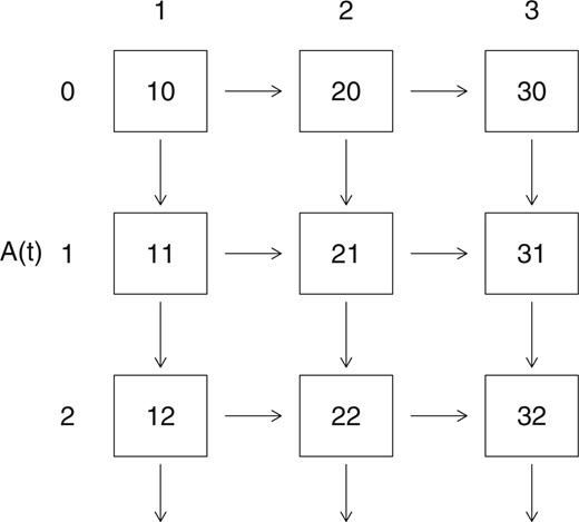
A state-space diagram for a joint model for a 3-state progressive life history process and a visit process.
Consider the joint process |$W(t) = (Z(t), A(t))$| with states |$(k, a)$| described above. We do not discuss covariates explicitly unless it is necessary but they are included in the process histories. We assume they are either defined functions of time or if random and time-varying, constant between visit times. This reflects the fact that time-varying covariates are typically observed just at visit times; we discuss this further below and in Section 5. To specify the joint process, we require intensities
where |$N_{kl}(t),t > 0$| counts the number of |$k$| to |$l$| transitions |$(k \ne l)$| in the life history process and as in the preceding sections, |$\bar{H}(t^-) = \{ \bar{Z}(t^{-}), \bar{A}(t^{-}), \bar{Y}(t^{-}), X \}$|. For a CIVP as defined in (2.2) the restriction on |$\lambda^{A}(t \mid \bar{H}(t^-))$| is
In addition, we require that (2.3) hold, or that
where |$\{N(t),t > 0\}$| denotes the multivariate counting process comprising counting processes for all types of life history transitions. A sufficient condition for this is that
where we recall that |$H(t^-)=\{Z(s),X(s),0 \le s < t\}$|. We reiterate that the time-varying covariates we consider are defined functions of time, or covariates that only change value and are measured at visit times. Defined time-dependent covariates could be month, or season, for example. Covariates that represent interventions at visit times often change value only at these times. For more general covariates that change in continuous time, a common approach is to assume that the most recently recorded values are adequate to model the multistate process of interest, and this is equivalent to assuming the covariates are constant between visits. As noted above, this can be problematic, especially when there are long gaps between visits.
Assumptions about the forms of intensities are needed to proceed with either the general model or CIVP cases. Lange and others (2015) considered a joint model for the life history process of interest and the visit process, with visit intensities that depends on the current life history state; they refer to these as disease-driven visits. They considered a time-homogeneous Markov model with intensities
as well as an extension where the life history intensities have a specific semi-Markov form. Since the visit intensity at |$t$| depends on the |$Z$|-state occupied at that time, the CIVP assumption in (2.8) is not satisfied so this is a non-CIVP (or conditionally dependent visit process) model. The model makes strong assumptions and is too simplistic for many settings, but it provides a convenient basis for discussion of the issues involved in joint modeling; more flexible non-homogeneous Markov models can also be considered. Transition and state entry time probabilities are easily calculated for the time-homogeneous model (2.10). In particular, if we order the states as |$\{(1,0)$|, |$(2,0)$|, |$\ldots$|, |$(K, 0);$||$(1,1)$|, |$(2,1)$|, |$\ldots$|, |$(K,1);$||$(1,2)$|, |$(2,2)$|, |$\ldots$|, |$(K, 2);$||$\ldots \}$| the transition intensity matrix for the joint process has block form
where |$Q$| is a |$K \times K$| matrix with |$q_{kl}$| in entry |$(k,l)$| and |$-\sum_{l \neq k} q_{k l}$| in the |$(k,k)$| diagonal entry, |$k,l = 1, \ldots, K$|, and |$\Lambda = {\rm diag}( \alpha_1, \ldots \alpha_K)$|. Transition probabilities can be calculated using the matrix exponential relationship |$P(t)=\exp(Rt)$|, where |$P(t)$| is the transition probability matrix (e.g. Kalbfleisch and Lawless, 1985; Jackson, 2011). Lange and others (2015) also considered a semi-Markov model for the life history process with phase-type state sojourn distributions by using a latent underlying Markov process (Titman and Sharples, 2010). In settings where inter-visit times can be fairly long, however, such models often involve estimability problems unless strong restrictions are made on the latent process. Alternative semi-Markov visit intensities, which may depend on the time since the last visit or the time since entry to the current disease state, are also problematic since the entry times to life history states are typically unobserved. We focus on (2.10) and non-homogeneous Markov models which are more plausible than semi-Markov models in many settings. However, in later sections, we consider semi-Markov models and in Section 4 and the Supplementary material available at Biostatistics online we show how they may be fitted. We now turn to likelihood construction with models that incorporate both disease-driven and conditionally independent visits.
2.3. Likelihood construction accommodating different visit types
For a typical individual, some visits may arise in a manner that is dependent on the current state of the life history process (i.e. be disease-driven) while others may occur at conditionally independent times. Lange and others (2015) categorize visits as disease-driven or scheduled, and assume that each separate visit can be classified as such; we adopt a similar framework to start. In modeling the disease-driven visit process, Lange and others (2015) conditioned on the observed scheduled visit times and treated them as censoring times for disease-driven visits. In practice, however, conditionally independent visit times are often random, and their intensity function may depend on information observed at the preceding visit as is permitted under (2.8). In this case, it is often of interest to examine the dependency of visit times on this information. Moreover, inverse-intensity-of-visit weighting (IIVW) and other weighting methods used for estimation of marginal or partially conditional models (e.g. Lin and others, 2004) require that visit intensities for a CIVP be modeled and estimated. We therefore consider explicitly the intensity for scheduled visits jointly with that for disease-driven visits. Visit processes may also be terminated by loss to follow-up. Thus we extend the joint model of Lange and others and take a competing risks approach to deal with these issues. Following visit |$j-1$| at time |$a_{j-1}$|, three outcomes are possible concerning the next visit: (i) the next visit may occur and be a scheduled visit; (ii) the next visit may occur and be a disease-driven visit; and (iii) the next visit may be censored by LTF. To formulate this, we define the three intensities |$\lambda^S(t|\bar{H}^{\circ}(t^-))$| for scheduled visits, |$\lambda^D(t|\bar{H}(t^-))$| for disease-driven visits, and |$\lambda^C(t|\bar{H}^{\circ}(t^-))$| for premature loss to follow-up (censoring). Follow-up may also terminate due to administrative censoring at time |$E$|; we treat |$E$| as a fixed (pre-specified) time. Note that scheduled visits and LTF are assumed to be conditionally independent by definition, with intensities that depend only on the observed process history |$\bar{H}^{\circ}(t^-)$| and that disease-driven visits are non-independent in general. We let |$A^{S}_j, A^{D}_j,$| and |$C$| denote potential scheduled visit, disease-driven visit, and censoring times, respectively, and define |$A_j=\min(A^S_j,A^D_j,\min(C,E))$|; we also let |$\Delta_j=I(A_j \ne \min(C,E))$| and |$\Delta^{D}_j=I(A_j=A^D_j)$|. We could at this point expand the state diagram for the joint model in Figure 2 to recognize these competing outcomes for the observation process but for simplicity we do not do this; instead, we will continue to use Figure 2 to portray potential states and possible transitions, but recognize that there are two types of visits (disease-driven and scheduled) and include the type of each visit in the process histories. That is, a downward transition in Figure 2, resulting from an event in the observation process, can be one of three types: a scheduled visit, a disease-driven visit, or observed LTF at time |$A_j$|. We note that when |$A_j$| is a LTF time (i.e. |$\Delta_j = 0$|), the state of the life history process at that time is unknown.
We can now give the form of the likelihood function based on observed data. Let |$A_j$| or |$ a_j$| denote the time of the |$j$|th visit or the LTF time and |$Z_j$| denote the state observed at that time, provided a visit occurs. Suppose for discussion that the information observed at a visit time |$a_j$| is just the state |$Z(a_j) = z_j$|. We consider the sequence |$(A_1, Z_1)$|, |$(A_2, Z_2)$|, |$\ldots$|, |$(A_m,Z_m)$| given |$A_0 = 0$| and |$z_0$|, where |$A_m$| is the time of the last observation or loss to follow-up time over |$(0,E]$|; if |$A_m$| is a LTF time then |$Z_m$| is unobserved. The likelihood contribution for an individual is then of the form |$L = L_1 \cdot L_2 \cdots L_m \cdot L_{m+1}$|, where each contribution is based on the event intensities for the life history, visit, and loss to follow-up processes as is conventional in event history analysis (Cook and Lawless, 2007; Aalen and others, 2008); the contribution |$L_{m+1}$| corresponds to the event that there are no further visits between |$a_m$| and |$\min(C,E)$|, along with the possible occurrence of random loss to follow-up over |$(a_m, E)$|. In the following, we focus on terms relevant for estimation of the life history and disease-driven process intensities; the intensities for independent (scheduled) visits and for LTF are for now treated as nuisance parameters unless specified otherwise. There are three types of likelihood contributions that provide information on the disease-driven visit process and life history process intensities; they depend on whether a visit at time |$a_j$| is type DD (disease-driven) or type S (scheduled), or whether |$a_j=\min(C,E)$|. We note that given |$C > a_{j-1}$| is part of |$\bar{H}^{\circ}(a_{j-1})$|, then |$A^S_j, A^D_j$|, and |$C$| are conditionally independent given |$\bar{H}^{\circ}(a_{j-1})$|.
If a disease-driven visit occurs at |$A_j$|, the likelihood contribution |$L_j$| takes the form
where for convenience we use “P” to represent either a probability density or mass function. Two transitions at the same time in the joint model are assumed impossible, and so this equals
where
and
Note that since we consider Markov models, |$\lambda^D(a_j | A_j \ge a_j, Z(a_j), \bar{H}^{\circ}(a_{j-1}))$| does not involve any transition times over |$(a_{j-1}, a_j)$|. The likelihood contribution for a scheduled visit is similarly
Finally, the likelihood contribution from LTF at time |$a_j=\min(C,E)$| is
since the state occupied at the LTF time is unknown.
Models can be fitted via maximum likelihood. The conditional independence of |$A^D_j$|, |$A^S_j$|, and |$C$| given |$\bar{H}^{\circ}(a_{j-1})$| allows each type of contribution to be evaluated as a product of separate terms involving (i) the joint model for the process of interest and the disease-driven visit process, (ii) the scheduled visit process intensity, and (iii) the censoring intensity. We typically ignore terms involving the censoring intensity, assuming they do not include any parameters in the disease-driven or life history process intensities (i.e. that censoring is non-informative). We may similarly ignore terms involving the scheduled visit intensity if our main objective is to estimate the disease-driven visit intensity and to address the effect of the outcome-dependent observation process. We would need to estimate the scheduled-visit intensity if IIVW estimation were of interest, but IIVW estimation is used under an assumption of a CIVP. In that case contributions for disease-driven visits are not present; the disease-driven intensities |$\lambda^A(t|\bar{H}(t^-))$| in (2.10) equal zero.
We ignore the terms |$\pi_j^S$| and |$\pi_j^C$| involving the scheduled visit and censoring intensities, and focus on the joint life history—disease-driven visits process. Note that the total visit intensity is the sum of the disease-driven and scheduled intensities (i.e. |$\lambda^A(t | \bar{H}(t^-)) = \lambda^D(t | \bar{H}(t^-)) + \lambda^S(t | \bar{H}^{\circ}(t^-))$|, so the visits process is a CIVP either if the disease-driven visit intensities are zero, or if they do not depend on |$\bar{H}(t^-)$| given |$\bar{H}^{\circ}(t^{-})$|. If every visit can be classified as disease-driven or scheduled, then the former condition is trivially determined by whether or not disease-driven visits occur. The latter case can be examined when a specific disease-driven model is adopted. In the present example, this corresponds to the condition |$\alpha_1=\alpha_2=\alpha_3$|. Finally, we note that likelihood contributions from a LTF time |$a_j$|, given by (2.15), are a little more complicated. We discuss this calculation in Section 3.
Although certain disease-driven visit models, such as the one in the preceding example, can be fitted to observed data, they cannot necessarily be easily checked. As we discuss in Section 3, we can check the CIVP condition |$\alpha_1 = \alpha_2 = \alpha_3$| within the time-homogeneous Markov model for disease-driven visits in Figure 2 and we can also fit non-homogeneous Markov models, but we cannot as readily assess the Markov assumption. Non-CIVP models require rather strong parametric assumptions to be tractable and estimable, and so their use needs to be considered cautiously. We also note that in many settings visits may not all be clearly classifiable as disease-driven or scheduled; we discuss this in Section 3. To further assess possible non-CIVP behavior, supplementary data are desirable. Classification of visits as scheduled or disease-driven is one type, and we discuss in Section 5 some other types that can facilitate assessment of the CIVP conditions. For example, this might take the form of more rigorous data collection so that visits can be more accurately classified as scheduled or disease-driven, or supplementary data on covariates that might be related to both visits and the life history process. In the next section, we consider estimation in Markov life history models in more detail and conduct numerical studies on the effect of assuming a CIVP when this is not true.
3. Estimation under Markov assumptions
3.1. Maximum likelihood estimation
Consider a time-homogeneous Markov model as in (2.10) and suppose interest lies in estimation of the parameters |$\theta$| that specify these intensities for life history transitions and disease-driven visits. We assume that the scheduled-visit and censoring intensities do not involve |$\theta$| and for convenience drop terms in the expressions (2.13)–(2.15) that involve them. From these expressions, the partial likelihood contribution for a scheduled or disease-driven visit at time |$A_j = a_j$| is proportional to
If |$A_j = a_j$| is a LTF time, the partial likelihood contribution is proportional to
For simplicity, we ignore covariates but when they are present we include values |$\bar{X}(a_{j-1})$| in |$\bar{H}^{\circ}(a_{j-1})$| and allow the visit and LTF times to depend on observed covariates. Transition probabilities needed in (3.1) and (3.2) are easily computed using matrix exponential functions. We observe first that, with states for |$(Z(t), A(t))$| in the joint model written in the order used in (2.11), we need only consider the reduced model with |$2K \times 2K$| transition intensity matrix |$R_0$| and transition probability matrix |$P(t)$|, given by
where |$P(t) = \exp(R_0 t)$|, which applies to calculations needed for every two successive visit times. The matrix |$P_1(t)$| required for (3.1) can be obtained by computing |$\exp(R_0 t)$| with |$t = a_j - a_{j-1}$|. The function expm in R or the function MatrixExp in the R msm package (Jackson, 2011) can be used to compute this matrix exponential. The calculation can be simplified since for a square matrix |$B$|, |$\exp(B) = \sum_{r=0}^{\infty} B^r/r!$|, so |$P_1(t) = \exp( (Q - \Lambda) \cdot t )$|, which only involves exponentiation of a |$K \times K$| matrix, rather than a |$2K \times 2K$| matrix.
The likelihood function from |$n$| independent joint life history and visit processes with visit times |$a_{ij}$|, |$j = 0, 1, \ldots, m_i$|, for process |$i$| and with |$a_{i m_i}$| assumed to be a random or administrative censoring time, is proportional to
where subscript |$i$| has been added to earlier expressions to denote individuals. This can be maximized using a general purpose optimizer such as the R optim or nlm functions on |$\log L(\theta)$|.
We have assumed that each visit can be correctly classified as a scheduled or disease-driven visit. This is feasible in clinical studies where, following a visit, the next scheduled-visit time may be assigned based on the status of the individual at the current visit. If this time is later adjusted for reasons unrelated to the disease process, the visit remains a scheduled visit. It is, however, good practice that during visits, information is obtained to allow accurate classification of the visit type; we discuss this further in Section 5. If |$\Delta_{ij}^D$| is sometimes unknown, we can maximize the resulting likelihood function directly or using an expectation–maximization algorithm (Dempster and others, 1977). This requires that the scheduled-visit intensity |$\lambda^S(t | \bar{H}^{\circ}(t^{-}))$| be modeled and estimated. In particular if we let |$R_{ij} = I(\Delta_j^D~\mbox{is known})$| for |$j=1,\ldots, m_i-1$|, the observed data likelihood can be given as follows for the time-homogeneous framework we have considered. For convenience, we write terms in (3.4) involving transition probabilities as
for |$j= 1, \ldots, m_i-1$| and
We assume that scheduled visits have intensities |$\alpha_k^S$| that depend on the last observed state. Then, accommodating the possibility of an unknown visit type, the observed data likelihood is
where |$\theta$| consists of the parameters |$\lambda_{rs}$|, |$\alpha_r,$| and |$\alpha^S$| consists of the |$\alpha^S_{r}$|. We note that if all |$R_{ij}=0$| then all parameters cannot be estimated from (3.5); we discuss this further in the Supplementary material available at Biostatistics online.
The time-homogeneous Markov model does not allow time trends in the intensity functions and is too simplistic for many situations. The development here can readily be extended to deal with non-homogeneous processes where the intensities in (2.10) are replaced with |$q_{k l}(t)$| and |$\alpha_{Z(t^{-})}(t)$|. In this case, the calculation of transition probabilities needed for (3.1) and (3.2) is slightly more complicated. Instead of matrices |$R_0$| and |$P(t)$| in (3.3), we consider
The transition probability matrix |$P(s,t)$| is given by the matrix product integral formula (Cook and Lawless, 2018, p. 36)
where |$s = u_0 < u_1 < \cdots < u_M = t$| is a partition of |$(s,t]$|, |$\Delta u_{\ell} = u_{\ell} - u_{\ell - 1}$| and all |$\Delta u_{\ell} \rightarrow 0$| as |$M \rightarrow \infty$|. The right-most product in (3.7) with |$M$| as small as 10 or 20 usually provides fast and sufficiently accurate computation of transition probabilities. As in the time-homogeneous case, it can be seen that in order to obtain |$P_1(s,t)$|, we can in fact use only the |$K \times K$| matrix |$Q(u) - \Lambda(u)$| in place of |$R_0(u)$| in (3.7).
It is recommended that some type of non-homogeneous model be fitted as a check on homogeneous models. Joint Markov models with piecewise-constant intensities are particularly useful (e.g. Cook and Lawless, 2014, 2018), and the msm function can be used for fitting such models. Sometimes Markov intensities are implausible as, for example, when the intensities for a certain state depend strongly on the time since entry to that state. Such models are difficult to fit when state entry times are unobserved, and so except for the case of progressive processes, which we consider in Section C of the Supplementary material available at Biostatistics online, most analyses use parametric Markov models.
We next report on numerical studies of estimation under both CIVP and joint modeling assumptions.
3.2. Numerical studies
Here, we consider some scenarios for two life history models: Model 1 is a 2-state alternating (reversible) model shown in Figure 1(c) and Model 2 is a 3-state progressive model as in Figure 1(d). The first scenarios considered involve time-homogeneous transition intensities, as follows:
Model 1: A 2-state alternating process with |$\lambda_{12} = 1$|, |$\lambda_{21} = 5$|, |$\alpha_1 = 0.5$|, |$\alpha_2 = 5$|
Model 2: A 3-state progressive process with |$\lambda_{12} = 1$|, |$\lambda_{23} = 5$|, |$\alpha_1 = 0.5$|, |$\alpha_2 = \alpha_3 = 5$|
Model 1 represents a setting with recurrent sojourns in state 2 of a fairly short duration relative to those of state 1 while Model 2 represents a progressive condition with the |$2 \rightarrow 3$| transition occurring at a much higher rate than the |$1 \rightarrow 2$| transition. For each model, the visit process intensities reflect the setting where we assume that if the |$(j-1)$|th visit occurs at time |$a_{j-1}$| and the state occupied then is |$z_{j-1}$|, then a potential scheduled visit is scheduled at a fixed time |$a_{j-1} + d_{z_{j-1}}$|. The visit occurs at this time only if no disease-driven visit occurs first; otherwise |$A_j$| is the time of the disease-driven visit. For both models, a disease-driven visit is much more likely if an individual is not in state 1. For simplicity, we used |$d_1 = d_2 = 0.5$| for Model 1 and |$d_1 = d_2 = d_3 = 0.5$| for Model 2. Cases with different schedules for each state gave similar results and are discussed below. We do not consider early loss to follow-up for simplicity but assume an administrative censoring time |$E = 5$|. In all cases we assume |$a_0=0$|. With the transition intensities given above, for Model 1 about 36% and 66% of the visits are disease-driven when the state at the preceding visit is 1 and 2, respectively. For Model 2, about 41% and 92% of the visits are disease-driven when the individual is in states 1 and 2 at the previous visit. Note that for Model 2, an individual’s follow-up continues after they enter state 3. We examine the performance of estimators of transition intensities under a CIVP assumption and under the joint model represented in (2.10) and (2.11). We also ran simulations for life history processes involving a covariate. We let |$\lambda_{kl}(x) = \lambda_{kl} \exp(\beta_{kl} x)$| with |$kl \in \{12, 21 \}$| for Model 1 and |$kl \in \{12, 23\}$| for Model 2. We set |$P(X = 1) = P(X = 0) = 0.5$| and |$\beta_{12} = 1.2$| for both models and |$\beta_{21} = 0$| and |$\beta_{23} = 0$| for Models 1 and 2, respectively. Values of all other parameters are the same as in the case without covariates and the values of |$d_k$| were also the same. The likelihoods (3.8) and (3.4) were maximized using the nlm function in R and the standard errors were computed based on the observed information matrix; confidence intervals (CIs) were based on the normal approximations for |$\log \widehat{\lambda}_{rs}$| and |$\log \widehat{\alpha}_r$|. In Table 1, we show results for each setting from 500 simulations involving samples of |$n = 1000$| individuals which is typical of many observational disease cohorts. We report for each estimator the empirical bias (EBIAS), the empirical standard error (ESE), the average standard error based on the observed information matrix (ASE), and the empirical coverage probability (ECP%) for nominal 95% CIs.
| Likelihood (3.8)—CIVP | Likelihood (3.4)—Joint model | |||||||||
|---|---|---|---|---|---|---|---|---|---|---|
| Value | EBIAS | ESE | ASE | ECP% | EBIAS | ESE | ASE | ECP% | ||
| 2-state model | ||||||||||
| |$\log \lambda_{12}$| | 0.0000 | 0.2839 | 0.0322 | 0.0345 | 0.0 | 0.0013 | 0.0279 | 0.0290 | 96.2 | |
| |$\log \lambda_{21}$| | 1.6094 | −0.3039 | 0.0292 | 0.0317 | 0.0 | 0.0001 | 0.0363 | 0.0365 | 95.6 | |
| |$\log \alpha_1$| | −0.6931 | — | — | — | — | −0.0006 | 0.0218 | 0.0220 | 95.2 | |
| |$\log \alpha_2$| | 1.6094 | — | — | — | — | −0.0002 | 0.0224 | 0.0219 | 94.0 | |
| 2-state model with covariates | ||||||||||
| |$\log \lambda_{12}$| | 0.0000 | 0.2823 | 0.0481 | 0.0489 | 0.0 | 0.0005 | 0.0408 | 0.0411 | 95.2 | |
| |$\log \lambda_{21}$| | 1.6094 | −0.3025 | 0.0432 | 0.0448 | 0.0 | 0.0025 | 0.0489 | 0.0489 | 94.2 | |
| |$\beta_{12}$| | 1.2000 | 0.0205 | 0.0699 | 0.0718 | 94.0 | 0.0014 | 0.0545 | 0.0557 | 95.6 | |
| |$\beta_{21}$| | 0.0000 | −0.1912 | 0.0614 | 0.0648 | 14.0 | −0.0034 | 0.0635 | 0.0664 | 95.4 | |
| |$\log \alpha_1$| | −0.6931 | — | — | — | — | −0.0012 | 0.0235 | 0.0240 | 96.2 | |
| |$\log \alpha_2$| | 1.6094 | — | — | — | — | −0.0009 | 0.0168 | 0.0174 | 95.2 | |
| 3-state model | ||||||||||
| |$\log \lambda_{12}$| | 0.0000 | 0.0506 | 0.0356 | 0.0319 | 66.6 | 0.0022 | 0.0340 | 0.0319 | 92.2 | |
| |$\log \lambda_{23}$| | 1.6094 | −0.1687 | 0.0331 | 0.0361 | 0.2 | −0.0016 | 0.0384 | 0.0383 | 95.6 | |
| |$\log \alpha_1$| | −0.6931 | — | — | — | — | −0.0033 | 0.0476 | 0.0451 | 94.4 | |
| |$\log \alpha_2$| | 1.6094 | — | — | — | — | −0.0014 | 0.0392 | 0.0383 | 93.6 | |
| |$\log \alpha_3$| | 1.6094 | — | — | — | — | −0.0006 | 0.0074 | 0.0073 | 95.2 | |
| 3-state model with covariates | ||||||||||
| |$\log \lambda_{12}$| | 0.0000 | 0.0517 | 0.0467 | 0.0452 | 80.4 | 0.0031 | 0.0446 | 0.0451 | 95.2 | |
| |$\log \lambda_{23}$| | 1.6094 | −0.1704 | 0.0478 | 0.0511 | 8.2 | −0.0031 | 0.0549 | 0.0529 | 93.6 | |
| |$\beta_{12}$| | 1.2000 | 0.1175 | 0.0722 | 0.0661 | 55.2 | −0.0037 | 0.0643 | 0.0653 | 95.4 | |
| |$\beta_{23}$| | 0.0000 | −0.0010 | 0.0676 | 0.0720 | 96.8 | 0.0018 | 0.0753 | 0.0728 | 93.8 | |
| |$\log \alpha_1$| | −0.6931 | — | — | — | — | −0.0034 | 0.0576 | 0.0560 | 93.0 | |
| |$\log \alpha_2$| | 1.6094 | — | — | — | — | −0.0008 | 0.0391 | 0.0384 | 95.4 | |
| |$\log \alpha_3$| | 1.6094 | — | — | — | — | −0.0006 | 0.0069 | 0.0070 | 95.6 | |
The left column of Table 1 shows the results of fitting models under the CIVP likelihood function (2.6), which, for a random sample of |$n$| individuals, becomes
where |$\lambda$| denotes the set of transition intensities |$\lambda_{rs}$|; the form is the same with the introduction of a covariate with the addition of conditioning on |$X$|. We assume, as in (3.4), that |$a_{i, m_i-1}$| is the last observed visit time for individual |$i$|, and that |$a_{i, m_i}$| is the censoring time, here equal to |$E = 5$|. The right column of Table 1 contains the results for the likelihood function (3.4), which accounts for disease-driven visits. The 2-state results are in the top half of the table and the 3-state results are in the bottom half.
The results under the CIVP assumption show that with disease-driven visits whose intensity varies across disease states, estimation of the disease process intensities and associated covariate effects is severely biased. Estimation using the joint disease process—disease-driven visits model, however produces valid estimates with minimal bias, and the empirical coverage for nominal 95% CIs is generally within the expected range.
We also ran simulations for other scenarios. When scheduled visit times depended on the last known state (with state 2 in Model 1 and states 2, 3 in Model 2 having shorter times to the next scheduled visit), results were similar to those in Table 1. We also investigated estimation using nonhomogeneous piecewise-constant transition intensities |$\lambda_{rs}(t)$| for the 3-state Model 2; these are reported in Table 2 and show features similar to those of Table 1. Simulations with intensities of “Weibull” form |$\lambda_{rs0}t^{\lambda_{rs1}}$| also gave similar results.
| Likelihood (3.8)—CIVP | Likelihood (3.4)—Joint model | |||||||||
|---|---|---|---|---|---|---|---|---|---|---|
| Interval | Value | EBIAS | ESE | ASE | ECP% | EBIAS | ESE | ASE | ECP% | |
| |$\log \lambda_{12}$| | |$[0, 2.5]$| | 0.0000 | 0.0525 | 0.0362 | 0.0332 | 67.8 | 0.0017 | 0.0347 | 0.0332 | 93.4 |
| |$(2.5, 5]$| | 0.0000 | 0.0288 | 0.1301 | 0.1218 | 92.6 | 0.0103 | 0.1265 | 0.1192 | 93.4 | |
| |$\log \lambda_{23}$| | |$[0, 2.5]$| | 1.6094 | −0.1728 | 0.0363 | 0.0381 | 0.4 | −0.0024 | 0.0423 | 0.0405 | 93.4 |
| |$(2.5, 5]$| | 1.6094 | −0.1231 | 0.1124 | 0.1197 | 83.2 | 0.0165 | 0.1289 | 0.1251 | 95.0 | |
| |$\log \alpha_1$| | |$[0, 2.5]$| | −0.6931 | — | — | — | — | −0.0031 | 0.0494 | 0.0469 | 94.6 |
| |$(2.5, 5]$| | −0.6931 | — | — | — | — | −0.0199 | 0.1814 | 0.1677 | 94.0 | |
| |$\log \alpha_2$| | |$[0, 2.5]$| | 1.6094 | — | — | — | — | −0.0016 | 0.0409 | 0.0404 | 94.4 |
| |$(2.5, 5]$| | 1.6094 | — | — | — | — | −0.0016 | 0.1289 | 0.1243 | 95.2 | |
| |$\log \alpha_3$| | |$[0, 2.5]$| | 1.6094 | — | — | — | — | −0.0010 | 0.0120 | 0.0121 | 96.2 |
| |$(2.5, 5]$| | 1.6094 | — | — | — | — | −0.0004 | 0.0092 | 0.0091 | 95.0 | |
Finally, we consider the case where scheduled visits also arise according to a intensity determined by the state occupied at the preceding visit; we denote these by |$\alpha_k^S$| where |$k$| denotes the state at the preceding visit. We considered Models 1 and 2 described above, with time-homogeneous scheduled visit intensities |$\alpha_1^S$|, |$\alpha_2^S$| for Model 1 and |$\alpha_1^S$|, |$\alpha_2^S$|, |$\alpha_3^S$| for Model 2. We investigate the situation in which some of the values |$\Delta_{ij}^{D}$| that indicate whether a visit is disease-driven (DD) or scheduled (S) are missing. We note that if all |$\Delta^D_{ij}$| are missing, model parameters can be non-identifiable, and such cases are excluded in the scenarios we consider. Specifically, we randomly assigned individuals to a sub-cohort in which they provide the reason for the visits when they occur so in this case |$R_{ij} = R_i$|, |$j = 1, \ldots$|. Those not in the sub-cohort did not provide this information. We considered the situation where |$P(R_i = 1) = 1.0$|, in which case data are complete on the cause for all visits, and where |$P(R_i=1)=0.25$| so that 75% of individuals do not furnish these data. Estimates were obtained by maximizing the likelihood (3.5) accommodating incomplete data on the nature of the visit.
In Table 3, we see that when only 25% of individuals had known visit type indicators, standard errors were, as expected, larger than when the types of all visits are known. Interestingly there is a very modest impact on the precision of the estimators of the transition intensities |$\lambda_{rs}$| for the disease process when only partial information is available on the nature of the visits. The parameters most affected by the incomplete information are the parameters of the visit processes. A caution concerning these results is that they depend on the assumed parametric models. When the visit type indicators are missing, our ability to check assumptions by generalizing the specification of the intensity functions is more limited. In Section 4, we consider a real setting involving a chronic disease cohort, and discuss some of the limitations imposed by the available data.
Estimates for the two- and three-state models obtained from likelihood (3.5) with complete and incomplete information on the nature of visit; |$E = 5$|, |$n = 1000$|, |$nsim = 500$|
| |$P(R_i = 1) = 1.0$| | |$P(R_i = 1) = 0.25$| | ||||||
|---|---|---|---|---|---|---|---|
| Value | EBIAS | ESE | ASE | EBIAS | ESE | ASE | |
| 2-state model | |||||||
| |$\log \lambda_{12}$| | 0.0000 | −0.0008 | 0.0261 | 0.0269 | −0.0007 | 0.0263 | 0.0271 |
| |$\log \lambda_{21}$| | 1.6094 | 0.0018 | 0.0311 | 0.0299 | 0.0014 | 0.0323 | 0.0308 |
| |$\log \alpha_1$| | −0.6931 | −0.0009 | 0.0220 | 0.0220 | 0.0039 | 0.0399 | 0.0402 |
| |$\log \alpha_2$| | 1.6094 | −0.0003 | 0.0212 | 0.0208 | −0.0008 | 0.0287 | 0.0283 |
| |$\log \alpha_1^S$| | 0.6931 | 0.0000 | 0.0112 | 0.0115 | −0.0013 | 0.0133 | 0.0144 |
| |$\log \alpha_2^S$| | 0.6931 | −0.0005 | 0.0199 | 0.0203 | −0.0010 | 0.0255 | 0.0267 |
| 3-state model | |||||||
| |$\log \lambda_{12}$| | 0.0000 | −0.0003 | 0.0314 | 0.0320 | −0.0002 | 0.0315 | 0.0320 |
| |$\log \lambda_{23}$| | 1.6094 | 0.0030 | 0.0377 | 0.0380 | 0.0024 | 0.0379 | 0.0392 |
| |$\log \alpha_1$| | −0.6931 | −0.0021 | 0.0430 | 0.0451 | −0.0006 | 0.0777 | 0.0828 |
| |$\log \alpha_2$| | 1.6094 | 0.0000 | 0.0379 | 0.0380 | −0.0023 | 0.0486 | 0.0505 |
| |$\log \alpha_3$| | 1.6094 | −0.0004 | 0.0073 | 0.0073 | −0.0007 | 0.0099 | 0.0099 |
| |$\log \alpha_{1}^S$| | 0.6931 | −0.0007 | 0.0212 | 0.0210 | −0.0015 | 0.0289 | 0.0272 |
| |$\log \alpha_{2}^S$| | 0.6931 | −0.0027 | 0.0518 | 0.0504 | −0.0015 | 0.0820 | 0.0818 |
| |$\log \alpha_{3}^S$| | 0.6931 | −0.0009 | 0.0122 | 0.0117 | −0.0004 | 0.0215 | 0.0206 |
There are several factors that influence the magnitude of the biases of estimators from analyses based on a CIVP assumption. First, in the context of the models of this section, the relative size of the state-dependent disease-driven visit intensities is a key aspect. However, the net risk of a disease-driven visit being realized (in light of the competing risk for scheduled visits) also matters; a strongly dependent disease-driven visit process in settings where conditionally independent scheduled visits occur more frequently will not result in much bias. In the simulations of Tables 1 to 3, the state-dependent visit intensities were ten-fold higher for some states compared to others and biases were large. Second, some parameters are affected by conditionally dependent visit processes more than others. Intensities and some functions of the intensities such as transition probabilities or state occupancy probabilities seem more sensitive than covariate effects. The weaker sensitivity of regression coefficients to dependently incomplete data has been observed in longitudinal settings with drop-out and survival analysis with dependent right censoring. Third, the nature of the underlying process (e.g. reversible as in Model 1 versus progressive as in Model 2) plays an important role; reversible processes are more susceptible to bias from state-dependent visits than progressive processes. Fourth, the number of covariates considered in the life history model is also a factor—the more covariates are controlled for the weaker the conditional independence assumption of a CIVP analysis. A fifth factor could be the percentage of visits of a known type (disease-driven or scheduled). Each of these points are useful to bear in mind when examining the results in the application in Section 4.
We report in Section B of the Supplementary material available at Biostatistics online on the results of further numerical studies of the impact of misspecification of the disease-driven visit intensity. In particular, we consider semi-Markov disease-driven visit intensities when the time-scale is the time since entry to the current disease state (Section B.1 of the Supplementary material available at Biostatistics online) and when it is the time since the most recent visit (Section B.2 of the Supplementary material available at Biostatistics online); in both settings the Markov assumption is invalid. We report on the empirical properties of estimators obtained from assuming a CIVP process and from joint modeling under the Markov disease-driven visit process. We find that estimators of the life history intensities and covariate effects are biased when the visit process is misspecified. Estimators of covariate effects are less affected than those of baseline intensities, and when the degree of misspecification is mild, biases may not be too large. This raises the issue of how models can be assessed for adequacy. We show in Section C of the Supplementary material available at Biostatistics online how a joint model with semi-Markov disease-driven visits can be fitted for the case of a progressive life history process. Fitting more complex models is difficult, however, and in these cases more frequent scheduled visits are recommended.
4. Modeling of severe joint damage in psoriatic arthritis
Here, we report on the analysis of data from the University of Toronto Psoriatic Arthritis cohort, a registry of patients which was launched in 1977 and is now comprised of over 1800 individuals. Patients are examined according to a formal protocol with clinic visits scheduled annually and radiographic examinations scheduled to take place every 2 years. At clinic visits, 64 joints of the hands, feet, and elsewhere are assessed and classified as severely damaged or not. The present goal is to predict the onset of a severe form of arthritis defined here as the presence of 3 or more severely damaged joints; this outcome is similar to an outcome termed arthritis mutilans based on radiological assessment of damage. To do this, we consider a four-state progressive model with states 1–4 representing zero damaged joints, and 1, 2, or 3 or more damaged joints, respectively. We take the time of diagnosis with PsA as the time origin since this represents the onset of disease activity, and assume |$Z(0) = 1$|. We restrict attention in this analysis to patients who were diagnosed with PsA in 1990 or later in order to confine attention to a period of time when the care of patients was relatively consistent, and select those recruited to the clinic within 5 years of diagnosis. Finally, we condition on |$A_0 = a_0$|, the time of the first clinic visit, and |$Z(a_0)$|.
In this clinic registry, visits are not classified as scheduled or disease-driven, so for illustration we adopt the following procedure to label them retrospectively. Since clinic visits are scheduled annually, if a visit occurs within 18 months of the previous visit (allowing for a 6-month appointment delay) it may be a scheduled visit, while visits after 18 months are designated disease-driven visits. At clinic visits blood tests are carried out to assess the level of inflammation based on the erythrocyte sedimentation rate (ESR). So if the ESR is measured and found to be above the normal value, we classify the visit as a disease-driven visit even if it is within 18 months of the prior visit. This post hoc approach to labeling visits is carried out as part of an illustrative analysis; while it is known that some visits are precipitated by a flare or other change in the disease condition, this information is not available. More satisfactory analyses would be possible if the clinic recorded the reason for the visit as we remark in Section 6.
Out of 4267 visits following a visit in which an individual was found to be in state 1, 1573 (36.9%) are designated as disease-driven according to this algorithm. Of the 310, 322, and 629 visits following a visit when the individual was in state 2, 3, or 4, 109 (35.2%), 101 (31.4%), and 232 (36.9%) were labeled as disease-driven, respectively. We consider analyses based on the four-state model fitted under the CIVP assumption, and analyses based on a joint model with state-specific disease-driven-visit intensities. We do not model the scheduled visit process because it is not of interest; this is justified under the assumption that LTF is conditionally independent of the life history, covariate, and visit processes.
We use piecewise-constant transition intensities for the four-state progressive response model with cut-points at 2.5, 5.0, 7.5, and 10 years; tests for the need for more cut-points to accommodate residual trend did not yield significant results. The results of fitting the four-state model under a CIVP assumption and a joint model with state-dependent disease-driven visit intensities are given in Table 4 for the case of no covariates. The disease-driven-visit intensities are assumed to be time-homogeneous, but time-dependent intensities can be accommodated. The null hypothesis of a CIVP can be assessed in the context of the joint model by testing the null hypothesis |$H_0$|: |$\alpha_1 = \alpha_2 = \alpha_3 = \alpha_4$| which would correspond to a state-independent “disease-driven” visit intensity. A likelihood ratio test of |$H_0$| gives |$p < 0.0001$| so there is very strong evidence against a CIVP; this is not surprising since the disease-driven visit intensities are estimated quite precisely and are increasing with the number of damaged joints. Interestingly, despite the fact that the CIVP process assumption is rejected there is only a small difference in the transition intensities for the response process estimated from fitting the four-state model under the CIVP assumption and the joint model; see the last paragraph in Section 3.2 for explanatory comments. We note that the hypothesis |$H_0$| corresponds to a CIVP sub-model within a specific joint model accommodating disease-driven visits; in general, CIVPs are not special cases of the disease-driven-visit model here. The small differences in CIVP estimates and joint model estimates may reflect the fact that the disease-driven-visit intensities, while different, do not vary as dramatically as in the simulation studies. In addition, only about one-third of the visits are designated as disease-driven.
Estimated transition intensities from a four-state progressive model with no covariates for the development of arthritis mutilans under a CIVP and a joint model with state-dependent visit intensities; time is measured in years
| CIVP Model | JOINT Model | |||||||||||
|---|---|---|---|---|---|---|---|---|---|---|---|---|
| Log intensity | Intensity | Log intensity | Intensity | |||||||||
| Transition | Interval | EST. | S.E. | EST. | 95% CI | EST. | S.E. | EST. | 95% CI | |||
| 4-state process | ||||||||||||
| |$1 \rightarrow 2$| | |$[0, 2.5)$| | −3.072 | 0.144 | 0.046 | (0.035, 0.061) | −3.099 | 0.144 | 0.045 | (0.034, 0.060) | |||
| |$[2.5, 5)$| | −3.351 | 0.206 | 0.035 | (0.023, 0.052) | −3.407 | 0.207 | 0.033 | (0.022, 0.050) | ||||
| |$[5, 7.5)$| | −3.283 | 0.239 | 0.037 | (0.023, 0.060) | −3.345 | 0.240 | 0.035 | (0.022, 0.056) | ||||
| |$[7.5, 10)$| | −3.377 | 0.297 | 0.034 | (0.019, 0.061) | −3.419 | 0.297 | 0.033 | (0.018, 0.059) | ||||
| |$[10, \infty)$| | −3.965 | 0.265 | 0.019 | (0.011, 0.032) | −4.011 | 0.266 | 0.018 | (0.011, 0.030) | ||||
| |$2 \rightarrow 3$| | |$[0, 2.5)$| | −0.348 | 0.219 | 0.706 | (0.459, 1.085) | −0.396 | 0.223 | 0.673 | (0.435, 1.043) | |||
| |$[2.5, 5)$| | −1.185 | 0.245 | 0.306 | (0.189, 0.494) | −1.241 | 0.248 | 0.289 | (0.178, 0.470) | ||||
| |$[5, 7.5)$| | −1.363 | 0.258 | 0.256 | (0.154, 0.425) | −1.417 | 0.261 | 0.242 | (0.145, 0.404) | ||||
| |$[7.5, 10)$| | −1.519 | 0.310 | 0.219 | (0.119, 0.402) | −1.579 | 0.314 | 0.206 | (0.111, 0.382) | ||||
| |$[10, \infty)$| | −2.055 | 0.289 | 0.128 | (0.073, 0.226) | −2.116 | 0.291 | 0.121 | (0.068, 0.213) | ||||
| |$3 \rightarrow 4$| | |$[0, 2.5)$| | −0.236 | 0.297 | 0.790 | (0.441, 1.413) | −0.261 | 0.303 | 0.770 | (0.425, 1.394) | |||
| |$[2.5, 5)$| | −0.626 | 0.290 | 0.535 | (0.303, 0.944) | −0.622 | 0.290 | 0.537 | (0.304, 0.948) | ||||
| |$[5, 7.5)$| | −1.087 | 0.325 | 0.337 | (0.178, 0.637) | −1.110 | 0.327 | 0.330 | (0.173, 0.626) | ||||
| |$[7.5, 10)$| | −1.864 | 0.461 | 0.155 | (0.063, 0.383) | −1.889 | 0.465 | 0.151 | (0.061, 0.376) | ||||
| |$[10, \infty)$| | −2.055 | 0.277 | 0.128 | (0.074, 0.220) | −2.071 | 0.278 | 0.126 | (0.073, 0.217) | ||||
| Visit process | ||||||||||||
| |$1 \rightarrow $| DD | — | — | — | — | −1.217 | 0.026 | 0.296 | (0.281, 0.312) | ||||
| |$2 \rightarrow $| DD | — | — | — | — | −1.099 | 0.094 | 0.333 | (0.277, 0.400) | ||||
| |$3 \rightarrow $| DD | — | — | — | — | −0.849 | 0.100 | 0.428 | (0.352, 0.521) | ||||
| |$4 \rightarrow $| DD | — | — | — | — | −0.690 | 0.064 | 0.501 | (0.442, 0.568) | ||||
DD, disease-driven visit.
In the first three panels of Figure 3, we display the estimates of the cumulative state entry time distributions based on the fitted four-state model and the joint model. Also displayed are nonparametric estimates of the marginal state entry time distributions obtained based on the interval-censored state entry times (Sun, 2006, Chapter 3). There is good agreement between the model-based and nonparametric estimates but we note that the non-parametric estimates are based on a stronger CIVP assumption that requires visit times to be completely independent of the damage process. The last panel of Figure 3 displays the estimates of the cumulative transition intensities from the joint model where it can be seen that the risk of damage for a first joint is considerably lower than the risk of progressive damage for a second and third joint; this is consistent with what is seen in the clinic where once a patient has developed damage in a joint the risk of future damage appears higher.
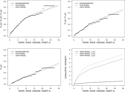
Estimates of the states 2, 3, and 4 entry time distributions from fitted four-state progressive Markov models in Table 4 with piecewise-constant transition intensities along with nonparametric estimates; also displayed are the cumulative transition intensity estimates from the joint model.
We next fit multiplicative intensity-based regression models for the transitions in the four-state model with intensities of the form
where |$X$| is a fixed |$p \times 1$| covariate vector, |$\beta_k$| is a |$p \times 1$| vector of regression coefficients, and |$\exp(\beta_{kj})$| is a relative risk for |$k \rightarrow k + 1$| transitions associated with a one unit increase in |$X_j$| when all other elements of |$X$| are held fixed. The covariates include an indicator of early disease onset (diagnosis by 40 years of age), status of the human leukocyte antigen HLA B27, an interaction between the early onset indicator and HLA B27 status, and sex. The model is fitted under the CIVP assumption and under the joint model and the estimated regression coefficients are reported in Table 5. There are very small differences in the estimated baseline intensities (not shown) and covariate effects under the four-state model fitted based on the CIVP assumption and the joint model; we note that in this setting the CIVP assumption for the four-state analysis is weaker than it is in the previous analysis due to conditioning on covariates. The likelihood ratio test of the CIVP assumption is again highly significant however.
Estimates obtained from fitting a four-state multiplicative intensity-based regression model reflecting the development of damage in psoriatic arthritis patients under the assumption of a CIVP and via a joint model with state-dependent intensities for disease-driven visits
| CIVP MODEL | JOINT MODEL | |||||||
|---|---|---|---|---|---|---|---|---|
| Covariate | Comparison | EST. | S.E. | p-value | EST. | S.E. | p-value | |
| Intensity for |$1 \rightarrow 2$| transitions | ||||||||
| Early onset | |${\le}40$| vs. |${>}40$| years | −0.644 | 0.199 | 0.0012 | −0.642 | 0.200 | 0.0013 | |
| HLA B27 | Yes vs. No | 0.377 | 0.338 | 0.2645 | 0.300 | 0.340 | 0.3779 | |
| Early onset |$\times$| HLA B27 | −0.194 | 0.534 | 0.7169 | −0.148 | 0.536 | 0.7826 | ||
| Sex | Female vs. male | 0.097 | 0.177 | 0.5836 | 0.076 | 0.178 | 0.6696 | |
| Intensity for |$2 \rightarrow 3$| transitions | ||||||||
| Early onset | |${\le}40$| vs. |${>}40$| years | −0.416 | 0.282 | 0.1402 | −0.453 | 0.286 | 0.1136 | |
| HLA B27 | Yes vs. No | 2.742 | 0.854 | 0.0013 | 2.902 | 0.916 | 0.0015 | |
| Early onset |$\times$| HLA B27 | −1.837 | 1.021 | 0.0721 | −2.093 | 1.088 | 0.0544 | ||
| Sex | Female vs. male | 0.559 | 0.244 | 0.0220 | 0.548 | 0.248 | 0.0273 | |
| Intensity for |$3 \rightarrow 4$| transitions | ||||||||
| Early onset | |${\le}40$| vs. |$>$|40 years | 0.572 | 0.341 | 0.0937 | 0.551 | 0.346 | 0.1109 | |
| HLA B27 | Yes vs. no | −0.577 | 0.505 | 0.2533 | −0.621 | 0.509 | 0.2222 | |
| Early onset |$\times$| HLA B27 | 1.775 | 0.782 | 0.0233 | 1.880 | 0.787 | 0.0170 | ||
| Sex | Female vs. male | 0.422 | 0.285 | 0.1385 | 0.423 | 0.288 | 0.1428 | |
The interaction between early onset and HLA B27 is significant for the |$3 \rightarrow 4$| transition intensity so we report on the effects of HLA B27 separately for those with early and late onset based on the joint model. The relative risks (RR) for a |$1 \rightarrow 2$| transition (first damaged joint) among HLA B27 positive versus negative individuals are RR = 1.164 (95% CI 0.518–2.618; |$p=0.713$|) and RR = 1.350 (95% CI 0.693–2.631; |$p=0.378$|) for those with early and late onset, respectively. The corresponding effects of early (versus late) onset are RR = 0.454 (95% CI 0.171–1.204; |$p=0.113$|) and RR = 0.526 (95% CI 0.356–0.779; |$p=0.001$|) for HLA B27 positive and negative individuals, respectively. Among individuals with two damaged joints, the effect of HLA B27 on the intensity for developing a third damaged joint is stronger for those with early onset (RR = 3.521; 95% CI 1.059–11.710; |$p=0.040$|) compared to those with late onset (RR = 0.537; 95% CI 0.198–1.457; |$p=0.222$|). The effect of early onset is likewise significantly different for those who are HLA B27 positive and negative with relative risks RR = 11.368 (95% CI 2.806–46.056; |$p<0.001$|) and RR = 1.735 (95% CI 0.881–3.415; |$p=0.111$|), respectively. Females have a significantly elevated rate of developing a second damaged joint compared to males (RR = 1.730; 95% CI 1.064–2.812; |$p=0.027$|) but there is little evidence of an effect for the other transitions. There is also little evidence of an effect of biologic therapy but we note that this will often be prescribed in individuals with a greater number of damaged joints than we consider here. Thus, positive HLA B27 status is associated with progression of damage. Interestingly, for those who are HLA B27 negative, early onset is associated with a lower risk for the first damaged joint.
In Section D of the Supplementary material available at Biostatistics online, we fit joint models with semi-Markov disease-driven visit intensities based on the likelihood constructed as described in Section C of the Supplementary material available at Biostatistics online; we use the time since the most recent visit as the time-scale for these intensities. While there is mild evidence of a small time-trend the parameter estimates for the disease process are very similar to those reported in Table 5.
5. Supplementary data and other considerations
It is good practice to compare inferences under CIVP assumptions with ones based on joint models allowing disease-driven visits. Although we can fit parametric joint models as shown in the preceding section, there is however no fully adequate way to check them, given the difficulty of fitting non-Markov models based on intermittent observation. Also, as the gaps between visits lengthen, information about parameters is reduced, even when each visit can be classified as a scheduled or disease-driven visit. In this section, we discuss some types of supplementary data that allow other checks on CIVP assumptions, and more detailed models to be fitted.
Supplementary data at visits. We have emphasized the common situation where states and covariates at the visit times are all that is known. However, with sufficient care, additional data may often be obtained, for example:
(i) individual-supplied reasons for the visit at |$a_j$|;
(ii) covariate information |$X(a_j)$| or in some cases, |$\bar{X}(a_{j-1},a_j)$| that may be related to visits and to the life history process;
(iii) information on the life history process |$Z(t)$| over |$(a_{j-1},a_j)$|.
Accurate information on life history or covariates between visit times may be hard to obtain and subject to measurement error. However, with the increased availability of monitoring technology, more information of this type is becoming available. We say more about this next.
Data collection between visits. If covariates |$X(t)$| that may be related to the life history and visit processes can be measured between visits, this information can be used to support more detailed modeling. In particular, we can include such information in the observed histories |$\bar{H}^{\circ}(t^-)$| and thus in the transition intensities |$\lambda_{kl}(t|\bar{H}^{\circ}(t^-))$|. It could also be used in models for the scheduled-visit intensity, as a basis for IIV weighted estimation (Cook and Lawless, 2018, Section 5.4), or for modeling the covariate process |$\{X(t), t \ge 0 \}$|; see for example Cook and Lawless (2018, Sections 5.2.1, 8.3). We remark that attempts to fit disease-driven-visit intensity models that involve covariates using only the data from observed visit times have been problematic, with likelihood maximization algorithms failing to converge. Additional information would be valuable for characterizing disease-driven-visit intensities.
Designated sub-cohorts. Sometimes a randomly selected sub-cohort of individuals can be chosen for more detailed data collection, including scheduled visits with rigorous adherence and accurate information about the reasons for any disease-driven visits. In this case, models fitted on this sub-cohort can be compared with models fitted on the remainder of the cohort, either with or without CIVP assumptions. The sub-cohort providing more detailed information can also be useful when assessing violations of the CIVP assumption for the full sample.
Tracing of individuals LTF. It often occurs that some individuals in a study cohort have not had a visit for a long time. In this case, we may decide to contact some or all of such individuals and with their agreement, schedule a visit. If information on the state then occupied and on certain covariates can be obtained, this can be compared with predictions based on models fitted under CIVP or non-CIVP assumptions. For the latter, we could also include in the last term in the likelihood (3.4) the information concerning |$Z(a_j)$|. In some cases, useful information may be obtainable without an actual visit.
Supplementary data and background knowledge about the life history process can help to identify and adjust for process-dependent visit times but as noted previously, models that incorporate disease-driven visits are difficult to check thoroughly even when visit types are accurately identified, because life history transition times are unknown. Nevertheless, the joint models provide additional insight and it is recommended that information on the reasons for visits be routinely collected.
6. Discussion
Much of the literature dealing with the relation between a disease process and a visit process has been based on shared or correlated random effect models (e.g. Liu and others, 2008); the same framework has been used extensively for modeling dependent censoring (e.g. Huang and Wolfe, 2002). When life history processes are under potential observation for a long period of time the simple dependence structure implied by such models is usually not realistic. The model proposed by Lange and others (2015) and studied here is designed to address this limitation and provide a more complete and powerful representation of the possible dependence structure. A particular advantage is the ability to accommodate state-dependence in the visit intensity which reflects the fact that changes in the disease state often precipitate clinic visits in chronic disease processes. When visits may arise for different reasons, some disease-related reasons may violate the independence assumptions implicit in standard analyses, but others may not; better analyses are possible if the reasons are recorded for at least some visits to ensure identifiability. As we discuss in Section A of the Supplementary material available at Biostatistics online, identifiability issues arise when there is no information about the reasons for visits.
Since the visit times are known, semi-Markov disease-driven visit intensities could be considered but fitting models and assessing intensities is challenging since they depend on the incompletely observed life history process. This leads to complex expressions for likelihood contributions as we demonstrate in Section C of the Supplementary material available at Biostatistics online. It helps a good deal if scheduled visits are not too far apart and we stress the desirability of this.
The joint models for the life history and visit processes we consider are discussed in the setting where LTF is conditionally independent of the life history, covariate, and visit processes given the observed history; moreover, we assume that the LTF time is non-informative. This simplifying assumption enabled us to focus attention on conditions of the visit process and relatively simple joint models. If the LTF time is not conditionally independent joint models of the life history and observation process will need to accommodate LTF and therefore become more complex. In ongoing work, we are studying such models but this is beyond the scope of the current paper.
We have also focused on the case in which all transitions of the life history process are unobserved due to intermittent examination of individuals. In many settings entry times to some (often absorbing) states are observable, subject only to right censoring. In chronic disease processes, entry to the absorbing state death can be observed and will terminate both the disease and visit processes. Adaptations of the models we consider to deal with this are relatively straightforward.
In some cohort studies, different types of information may be collected at different kinds of visits. Some visits may involve more intensive data collection and accurate examination of the disease status, while others may involve less expensive and less accurate classification of individuals. The University of Toronto Psoriatic Arthritis Clinic has a formal protocol in which patients are to undergo detailed annual clinical examination by a physician but are to be examined radiologically for joint damage only every second year. When the clinical examination yields a less accurate assessment of the disease state, some visits may provide misclassified designations. Hidden Markov models (Titman and Sharples, 2010) are useful when imperfect state classifications arise, but little work has been carried out on the setting where some visits may yield accurate designations and some inaccurate designations. Models accommodating disease-dependent visit processes could enhance information about the latent states in this case.
Delayed entry to a study, with an initial visit at time |$a_0>0$|, is readily accommodated provided sufficient information is available on the history |$H(a_0)$| to render the subsequent process independent of the delayed entry time. Such information will, for example, be crucial when using data from tertiary care centers since referral to such centers will typically occur when there has been either a prolonged period of uncontrolled disease activity or a sudden increase in it. In the absence of auxiliary data on unselected individuals, it is difficult to check the validity of any assumptions about conditionally independent delayed entry.
We have restricted attention to the case of fixed covariates, defined time-varying covariates, or time-varying covariates which change only at visit times; covariates which vary randomly in continuous time are more difficult to handle. Much of the work on joint modeling of longitudinal markers and failure times has been carried out to deal with this challenge using hierarchical linear models with shared or correlated random effects acting on the hazard function (Rizopoulos, 2012). Extensions accommodating more general life history processes are possible, but these models are primarily descriptive and do not provide a realistic representation of local dependence (Aalen and others, 2008), nor the effect of terminal events such as death (Cook and Lawless, 2018, Section 8.3). The conventional approach of “carrying forward” the most recently measured value of a marker to avoid a model for |$X(t)$|, can yield attenuated estimates of effects. Approaches geared towards addressing this attenuation include the aforementioned joint modeling approaches, smoothing covariate values (e.g. Raboud and others, 1993; Tsiatis and others, 1995), regression on the time since the most recent covariate measurement (e.g. de Bruijne and others, 2001), and regression calibration (Andersen and Liestol, 2003). There is much scope for further work on methods for handling time-varying covariates measured at conditionally independent or dependent visit times for general life history processes.
Funding
Natural Sciences and Engineering Research Council of Canada (RGPIN 155849 and RGPIN 04207 to R.J.C.; RGPIN 8597 to J.F.L.); and the Canadian Institutes of Health Research (FRN 13887 to R.J.C.).
Acknowledgments
Richard J. Cook is a Tier I Canada Research Chair in Statistical Methods for Health Research. The authors thank Drs Dafna Gladman, Vinod Chandra, and Lihi Eder for stimulating discussion regarding the University of Toronto Psoriatic Arthritis Registry and Ker-Ai Lee for assistance in the computing. Conflict of Interest: None declared.
