


SUMMARY
Two-phase sampling design is a common practice in many medical studies. Generally, the first-phase classification is fallible but relatively cheap, while the accurate second phase state-of-the-art medical diagnosis is complex and rather expensive to perform. When constructed efficiently it offers great potential for higher true case detection as well as for higher precision at a limited cost. In this article, we consider epidemiological studies with two-phase sampling design. However, instead of a single two-phase study, we consider a scenario where a series of two-phase studies are done in a longitudinal fashion on a cohort of interest. Another major design issue is non-curable pattern of certain disease (e.g. Dementia, Alzheimer’s etc.). Thus often the identified disease positive subjects are removed from the original population under observation, as they require clinical attention, which is quite different from the yet unidentified group. In this article, we motivated our methodology development from two real-life studies. We consider efficient and simultaneous estimation of prevalence as well incidence at multiple time points from a sampling design-based approach. We have explicitly shown the benefit of our developed methodology for an elderly population with significant burden of home-health care usage and at the high risk of major depressive disorder.
1. Introduction
The aim of any multi-phase design is of two-fold. First, to detect as many cases as possible and second, the efficient estimation of prevalence at a limited cost. Two-phase design in particular has been very popular in epidemiological studies (Pickels and others, 1995; Dunn and others, 1999). In a standard two-phase design (Neyman, 1938), at the first phase all subjects under study receive a low cost and easy to administer but fallible screening test. Depending upon the first phase result, subjects are then classified into two (or more) categories. In the second phase, a random sample is drawn from each of these categories, which undergoes state-of-the-art (or “gold-standard”) and rather expensive diagnostic procedure to determine their true disease status. Optimal design strategies for two-phase surveys has been discussed in Deming (1977), Shrout and Newman (1989) and McName (2004). For a more detailed review of the literature, please see Pickels and others (1995). Two-phase studies are popular in psychometric research and commonly found in mental health (Beckett and others, 1992; Hendrie and others, 2001) studies.
In the two-phase study the most important task is the estimation of prevalence, i.e. previously undetected and untreated “cases”. However, often we are presented with a scenario where multiple two-phase studies are performed over different time points. For such a scenario not only the prevalence but also estimation of the incidence, i.e. the frequency of the fresh cases, also becomes significant. In a regression estimation setup Clayton and others (1998) represented such a scenario. However that study has limitation in two senses. First, it focuses on the incidence estimation only and second, it only considers two time points. Extension of the same for multiple time points in the Longitudinal data framework is complicated and unexplored so far. In this article, we present simultaneous estimation of prevalence and incidence from the sampling design perspective. Our method is fairly simple and applicable for multiple time points.
1.1. Motivating example 1
Our first example comes from a NIH funded study for detecting Alzheimer and Dementia in two communities. The study design is presented in detail in Hendrie and others (1995, 2001). A fixed number of elderly subjects are followed in a longitudinal fashion for about 5 years in two communities (African Americans in Indiana, USA and Yoruba in Ibadan, Nigeria). The estimation of prevalence and incidence of dementia is carried out at two time points (or waves) separately at 2-year follow-up and at 5-year follow-up. However, due to irreversible nature of the disease, at each successive time point those who are identified to be demented via the second phase gold-standard test are progressively excluded. Hence, it represents a monotonic decreasing population under investigation over the time (see Figure 1(a)). Though new subjects could be included as part of the existing cohort, we did not consider those in the current context. At each wave a two-phase design is carried out. In the first phase, a screening test is done based on CSI’D’ score (Hall and others, 1999). Based on the output of this score subjects are categorized into four groups (Good, Intermediate, Poor, and Impaired). A random sample with fixed percentage from each category is drawn for second phase clinical assessment, which is considered to be gold-standard. An ethical sampling plan (see Section 2) is followed. The percentage to be sampled for second phase from each outcome group is not guided by any optimality property, rather based on associated cost and convenience. More importantly, the wave 1 and wave 2 estimations are carried out independently. There exist other interesting aspect of this cohort, which are studied in many subsequent papers (Callahan and others, 1996; Shen and others, 2006), but we do not elaborate further as that is not the main goal of this article.
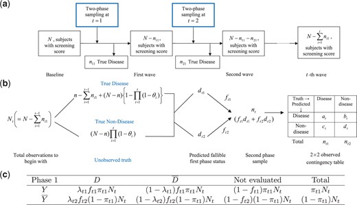
Schematic diagram of the longitudinal two-phase study in (a). Schematic diagram of the two-phase study at |$T=t$| in (b). Expected frequency in the cells of the survey at |$T=t$| are presented in (c).
1.2. Motivating example 2
Our second example comes from another NIH funded study to detect late life depression (LLD) in medical home care. LLD is under identified, under diagnosed and under treated. The identification of LLD is complicated due to co-morbid physical illness, impaired cognitive function, and stigma associate with being diagnosed as depressed at an older age. Thus the main goal of the study was to assess the prevalence, 1-month persistence and other clinical features, and clinical, functional, and health care outcomes at 12 months of major depression and subsyndromal depression in elderly patients newly admitted for medical home care at a large regional Visiting Nurses Agency (VNS Westchester County, NY, USA). The subjects were a random representative sample of elderly patients (age 65 or more) from primarily homebound newly admitted to the VNS and were sampled on a weekly basis for a period of 2 years. For this specific study two-phase sampling was not proposed originally, rather a single gold-standard test is carried out. A team of geriatric psychiatrist, geriatrician, clinical psychologist, and sociologist evaluated HAM-D, GDS, SCID (patient and informant), and tape recorded semi-structured Nurse interview together to create a new “gold-standard” of major depression that is based on consensus using DSM-IV diagnosis criteria (Bruce and others, 2002; Weinberger and others, 2009). Undoubtedly, this was time consuming and expensive, albeit followed DSM-IV’s “etiologic” approach for the diagnoses of depression. Though the primary end-point of the original study was 12 month, the data was collected at baseline, at 3-month and at the end of 12 month study period, however, subjects were followed over a 24-month period. Our objective in this present situation is to show that if a well constructed screening test was implemented using available surrogate information in a two-phase sampling design, one can estimate incidence and prevalence quite accurately but using a much smaller sample size (i.e. lower cost). This is because unlike the original study design, not all subjects were required to be evaluated in the gold-standard test even when an “Ethical” sampling plan is followed. There exist many other interesting aspect of this study from subject characteristics, which are studied in many subsequent papers (Weissman and others, 2011a,b).
In the rest of the article, we closely follow the common design of our motivating examples, though the methodological development is general enough to be applicable to any longitudinal two-phase sampling plan. The rest of the article is organized as follows. In Section 2, we introduce some notation and relevant background material. In Section 3, we discuss estimation issue for the incidence rate over time. We have done some efficiency analysis in Section 4, under the assumption that the cost of each phase is available. Section 5 concentrated on simulation studies with screening test improving/degrading over time. In Section 6, we have taken one of the motivating examples to study the behavior of our estimate. We conclude the article with a brief discussion.
2. Design of two-phase survey: some notations
First, we introduce some notations, which are broadly taken from Shrout and Newman (1989) as: |$D$|, true disease status (e.g. presence of diseases, for e.g. dementia, depression etc.) indicated by some well-defined diagnostic procedure; |$X$|, explanatory variable(s) (e.g. informants score, demographic, socioeconomic, and other subrogate information) used for predicting prevalence in phase one; |$Y$| the fallible classification obtained using screening test in phase one. In phase one based on |$X$|, we first classify the subjects either |$Y=1$| (presence of disease) or |$Y=2$| (absence of disease or, |$\overline{Y}$|). Popularly logistic regression have been used (Gao and others, 2000), however, the labeling of |$Y$| is more of a clustering problem than a classification one. This will be elucidated further in the simulation section. At the baseline, we have |$N$| many individuals in the study, out of whom |$n (<<N)$| have the disease. Of course |$n$| is unknown and need to be estimated. Let the random variable |$T=t$| denote the |$t$|-th two-phase study (also known as |$t$|-th wave) for |$T=1,2,3,\cdots$|, which are not necessarily equispaced. At |$T=t$|, let |$p_t$| denote the prevalence rate. For the transition from |$T=t-1$| to |$t$|, let |$\theta_{t}$| denote the incidence rate. At the baseline, i.e. when |$T=1$| our initial assumption is |$\theta_1=0$|, so one only have to estimate prevalence (|$p_1$|). For the sake of simplicity in this article we assume there is no loss due to death, absence etc., at different phases and also at different time points. Let |$n_{t1}$| and |$n_{t2}$| denote number of people for which we detect |$D=1$| and |$D=2$| (or, |$\overline{D}$|) at the second phase of |$T=t$|, respectively. Due to the irreversible nature of many disease (e.g. dementia, Alzheimer’s etc.) it is assumed that once accurate diagnosis is made (in the second phase), we exclude those people from the study at all other successive time points. Hence at the beginning of |$T=t$|, number of subject under study is |$N_t=N-\sum_{i=1}^{t-1} n_{i1}$|. Let |$d_{tj}=\sum_{i=1}^{N_t} 1_{\{Y_i = j|X_i\}}$| denote number of subject classified as |$Y=j$| for |$j=1, 2$|. Note that |$N_t= \sum_{j=1}^2 d_{tj}$| for |$\forall \ T=t$|. Following standard notion, let |$f_{tj}$| for |$j=1,2$| denote the fraction of the random sample included in the second phase study at |$T=t$|. If |$n_t$| is the number of second phase sample for |$T=t$| then |$n_t=\sum_{j=1}^2 f_{tj} d_{tj}$|. Due to “Ethical” reason (Shrout and Newman, 1989) in many two-phase studies |$f_{t1}=1$| is chosen or all the screened positive (|$Y=1$|) samples are included in the second phase. For our motivating example 1 this is the case, however for general discussion we will assume |$0\leq f_{tj}\leq 1$|, |$j=1,2$|.
3. Estimation of incidence rate
Prevalence is essentially the number of persons having true disease at the beginning of the study in the cohort or population of interest. At all other time points estimation of incidence is more important and meaningful. At those points prevalence has contribution both from the fresh cases of disease as well as from the previously undetected cases. A general outline of the above sampling design at |$T=t$| is presented in Figure 1(b), in which, the observed outcome of the first and second phase is depicted in a |$2\times2$| contingency table. The true unobserved disease status in Figure 1(b) requires some algebra and is given in Theorem 3.1 below.
Suppose we have |$N_t$| many subjects under the study at the beginning of |$T=t$|, with |$\theta_{t}$| being the incidence rate for the transition from |$T=t-1$| to |$T=t$|. Then the number of subjects with true disease is given by, |$n-\sum_{i=1}^{t-1}n_{i1}+(N-n)\left\{1- \prod_{i=1}^{t}(1-\theta_i)\right\}$|, while its complement is |$(N-n)\left\{\prod_{i=1}^{t}(1-\theta_i)\right\}$|.
An exact formula for the variance involving the product of many random variables are given in Goodman (1962). Unfortunately, even if we assume independence of the involving random variables, variance calculation for |${\theta}_{t}$| is rather prohibitive. Next, we present another equivalent formulation of |${\theta}_{t}$|, which is computationally much simpler.
3.1. Equivalent form for |$\theta_t$|
The interpretation of the above estimate is straight forward, which essentially is a ratio of the number of new cases of positive disease status, divided by the effective sample size at |$t$|-th time. Above estimate of |$\theta_t$| has some interesting property for “Ethical” sampling design (Shrout and Newman, 1989), depending upon the sensitivity of the first phase test, which is described below.
For the “Ethical” sampling design |$p_ t=\theta_t$|, if and only if sensitivity at the |$T=t-1$| is equal to |$1$|.
Equations (3.1) and (3.2) may look unrelated, but in fact they are equivalent. To show that we next propose a lemma.
Both the estimate of |$\theta_{t}$| given in equations (3.1) and 3.2 are equivalent in the sense that following identity connects them together,|$\prod_{i=1}^t (1-\theta_{t})=\frac{N_t (1-p_{t})}{N (1-p_{1})}.$|
4. Efficiency comparison: single- vs. two-phase design
4.1. Screening test improves over time
4.2. Screening test degrades over time
Hence the reduction in SE is bounded by, |$ 1-\frac{\mbox{min SE}_{2-phase}}{\mbox{SE}_{1-phase}}<1-\frac{2\sqrt{e^{-1/t}}}{1+e^{-1/t}}. $| The expression for the case |$S_{t1}\neq S_{t2}$| can be obtained in a similar fashion.
5. Simulation studies
As stated in the introduction section, our work is motivated by the problem of estimating incidence and prevalence in longitudinal setup. Two motivating examples have many common features (detection of disease status longitudinally), as well as variations, which are unique to each specific study design. In simulation setup, we have assumed a simplified setup which is common to both studies, to get a good idea how our estimation method performs under different scenario. In particular, we assumed that a fixed number of sample is being followed over the time, with no additional recruitment in between. There could be also data loss due to attrition and dropout due to untimely death and refusal to participate in the study at a future date. Missing data and time varying covariates are also often accompany many longitudinal study, however not considered in the present setup.
We assumed that the covariate(s) |$X$| which could be surrogate marker(s), informants score, socio/clinical variables etc. (e.g. CSI’D’ in example 1 of Hall and others (1999)) are used or potentially could be used in the actual study to do the stratification in the first phase. Prevalence and incidence are also could be highly correlated with other demographic variables such as age, sex, race etc. A logistic regression based classification technique has been used to create |$Y$| in Shen and others (2006). However, in the present case stratification of phase one is more of a clustering problem rather than the classification. Clustering essentially involves creating labels (|$Y$|) from the explanatory variable(s) (|$X$|), while classification aims to create “rules” when both |$Y$| and |$X$| are available. Unfortunately |$Y$| is not available in the present case in the beginning of phase one. Hence for the creation of |$Y$| label we have used mixture model based clustering (Fraley and Raftery, 2006) with two clusters (e.g. disease and non-disease) for all simulation. Details of the simulation steps are as follows:
We generate |$900$| samples for the non-disease group such that |$X_N\sim N(2,2)$|. For the disease positive group, we generate |$100$| samples from |$X_D\sim N(-2,4)$|. We store the original labels (disease and non-disease) as |$D$|. In the motivating example 1 (Hall and others, 1999), subjects with lower CSI’D’ are deemed to be demented and also the standard deviation in the demented group is higher than the normal one. Choice of |$X_D$| and |$X_N$| are primarily governed by the above considerations. Above distributional setup also ensures existence of enough overlap between two groups, thus creating some degree of fallibility in |$Y$|.
We cluster |$N=1000$| samples into two different clusters using mixture model. Denote |$Y_i=1$| if i-th subject is grouped in the disease positive cluster, |$2$| otherwise. Clustering acts as a proxy to the fallible phase one screening test in our simulation.
Following the strategy of Shrout and Newman (1989), select every member from the disease positive cluster and randomly select |$10\%$| subjects from the non-disease one.
On the assumption that gold-standard second phase test is highly accurate, treat the original |$D$| as the output of it. Create a |$2\times 2$| contingency table comparing |$Y$| and |$D$| of those subjects selected at the second phase. Estimate the prevalence and incidence rate (if applicable).
Remove those subjects who have had the true disease positive status in the second phase via |$D$|.
Choose a |$\theta_t$| (incidence rate) and out of |$N-n$| non-disease individuals change the status of |$(N-n)\theta_t$| many subjects from non-disease to disease. Note that, for variable incidence rate, |$\theta_t$| will vary for each |$T=t$|, while for the fixed |$\theta_t$| it needs to be selected only once. For those with changed status are assigned a new covariate |$X$| following Step 1.
The true number of the sample from each category can be found from the Figure 1(b) (see “Unobserved Truth”) as a function of time.
No more updating of the covariate |$X$| is needed if we assume that it is invariant over time. However, if we assume monotonic changes (improvement/degradation) in the |$X$|, adjustments are required. Improvements will signify further separation of disease and non-disease groups, resulting in more accurate prediction of |$Y$|. For each member in the disease positive group change the score of the |$i-$|th individual as, |$X_i^{new}=X_i^{old}-\delta_i \gamma_i$|, where |$\delta_i \sim U[0,2]$| denotes the rate of improvement and |$\gamma_i\sim Bernoulli(0.5)$| is an indicator of such an improvement. |$\delta_i$| and |$\gamma_i$| vary among different individuals. If we choose |$\gamma_i=1$|, |$\forall i$| it indicates improvement for all subjects, while for |$\gamma_i=0$|, |$\forall i$| indicates the invariant case. Similarly for the non-disease group define, |$X_i^{new}=X_i^{old}+\delta_i\gamma_i$|. For the degradation of informants score we will follow similar strategy by defining |$X_i^{new}=X_i^{old}+\delta_i\gamma_i$| for the disease positive group and |$X_i^{new}=X_i^{old}-\delta_i\gamma_i$| for the non-disease group. This essentially makes separation between two groups even harder, which in turn will lower the predictive accuracy of |$Y$|.
We repeat the above steps for |$T=1,2,\ldots,10$|. Note that our motivating examples have only few (two in example 1 and three in example 2) time points including the baseline. Here, we consider six different possible scenarios;
Time invariant |$X$| with fixed incidence rate.
Classification via |$X$| improves with time and fixed incidence rate.
Classification via |$X$| degrades with time and fixed incidence rate.
Time invariant |$X$| with variable incidence rate.
Classification via |$X$| improves with time and variable incidence rate.
Classification via |$X$| degrades with time and variable incidence rate.
For each case, we estimate the prevalence and incidence rate via equations (2.1) and (3.2) and also their respective variance. The result for six different cases are represented in Tables 1 and 2. In each table, we also report the sensitivity and specificity of the first phase clustering result. This is important as pointed out by McName (2003), as the efficiency of the two-phase design often determined by the high sensitivity and/or specificity. For the comparison purpose we also report the true prevalence, which is obtained via |$D$| in each wave. Table 1 represents the fixed incidence rate case with |$\theta_t=0.05$| for all the waves. For the time invariant |$X$|, the estimated incidence rate is close to the true value. When |$X$| improves in predicting |$Y$| with time, the estimated incidence rate is highly accurate and numerically very close to the true value |$0.05$|. We also see after wave five, the first phase clustering results are perfect with sensitivity and specificity approaching to one. While this is too good to be true in reality it does indicate the fact that sensitivity and specificity of the first phase test plays a significant role, not only in the efficiency of the two-phase design but also on the accuracy of the estimated incidence rate. Similar statements can be made on the estimate of the prevalence. On the other hand, when |$X$| degrades in predicting |$Y$| with time the first phase clustering produces many misclassified |$Y$|. This results in low sensitivity and specificity with progressing time. Notably, prevalence estimate is quite robust to withstand this mis-specification, however, similar statements cannot be made for the incidence estimate. Table 2 represents the variable incidence rate case. For the invariant case the results are not as accurate as the fixed incidence rate (see Table 1) for both |$p_t$| and |$\theta_t$|. However, if we compute the simple correlation between |$\widehat{\theta_t}$| and true |$\theta_t$| it yields correlation of |$0.91$|. Notably, the specificity for both tables are relatively low. For the improved |$X$| the estimates (for both |$p_t$| and |$\theta_t$|) are quite accurate, with high first phase sensitivity and specificity. Simulation studies presented above exhibits somewhat low specificity due to the non-separability between the disease and non-disease group resulting in high number of false positives. This can be easily altered by lowering the standard deviation each normal distribution. Additional results with high baseline specificity (and sensitivity) is available in the supplementary material available at Biostatistics online.
Simulation result for fixed |$\theta_t$| for three different scenarios
| Scenario 1: Time invariant |$X$| | ||||||||
|---|---|---|---|---|---|---|---|---|
| Time | |$\widehat{p_t}$| | V(|$\widehat{p_t}$|) | |$\widehat{\theta_t}$| | V(|$\widehat{\theta_t}$|) | Sensitivity | Specificity | True |$p_t$| | True |$\theta_t$| |
| Baseline | 0.0998 | 0.0162 | — | — | 0.975 | 0.178 | 0.1 | — |
| Wave1 | 0.0771 | 0.0194 | 0.0588 | 0.0259 | 0.932 | 0.114 | 0.068 | 0.05 |
| Wave2 | 0.0729 | 0.0202 | 0.0436 | 0.0281 | 0.919 | 0.143 | 0.07 | 0.05 |
| Wave3 | 0.0825 | 0.0213 | 0.0522 | 0.029 | 0.928 | 0.143 | 0.078 | 0.05 |
| Wave4 | 0.0704 | 0.0188 | 0.0376 | 0.0288 | 0.947 | 0.134 | 0.079 | 0.05 |
| Wave5 | 0.07 | 0.0196 | 0.0474 | 0.0272 | 0.943 | 0.136 | 0.082 | 0.05 |
| Wave6 | 0.0706 | 0.016 | 0.0468 | 0.0254 | 0.976 | 0.098 | 0.086 | 0.05 |
| Wave7 | 0.0734 | 0.0169 | 0.061 | 0.0233 | 0.975 | 0.073 | 0.078 | 0.05 |
| Wave8 | 0.0788 | 0.023 | 0.0657 | 0.0284 | 0.937 | 0.074 | 0.067 | 0.05 |
| Wave9 | 0.0641 | 0.0182 | 0.0349 | 0.0298 | 0.967 | 0.082 | 0.067 | 0.05 |
| Wave10 | 0.0843 | 0.025 | 0.0699 | 0.0303 | 0.935 | 0.087 | 0.067 | 0.05 |
| Scenario 2: Classification via |$X$| improves with time | ||||||||
| Baseline | 0.0998 | 0.0162 | — | — | 0.975 | 0.178 | 0.1 | — |
| Wave1 | 0.0879 | 0.0218 | 0.0698 | 0.0275 | 0.911 | 0.112 | 0.068 | 0.05 |
| Wave2 | 0.0812 | 0.0177 | 0.0421 | 0.0283 | 0.962 | 0.265 | 0.069 | 0.05 |
| Wave3 | 0.0646 | 0.0143 | 0.0437 | 0.0231 | 0.977 | 0.173 | 0.06 | 0.05 |
| Wave4 | 0.0631 | 0.0149 | 0.0522 | 0.0207 | 0.975 | 0.798 | 0.057 | 0.05 |
| Wave5 | 0.0489 | 0.0079 | 0.0371 | 0.0172 | 1 | 1 | 0.056 | 0.05 |
| Wave6 | 0.0557 | 0.0087 | 0.0557 | 0.0116 | 1 | 1 | 0.057 | 0.05 |
| Wave7 | 0.0514 | 0.0086 | 0.0514 | 0.0122 | 1 | 1 | 0.051 | 0.05 |
| Wave8 | 0.0462 | 0.0083 | 0.0462 | 0.0121 | 1 | 1 | 0.049 | 0.05 |
| Wave9 | 0.0535 | 0.0092 | 0.0535 | 0.0123 | 1 | 1 | 0.053 | 0.05 |
| Wave10 | 0.0494 | 0.0091 | 0.0494 | 0.013 | 1 | 1 | 0.049 | 0.05 |
| Scenario 3: Classification via |$X$| degrades with time | ||||||||
| Baseline | 0.092 | 0.0091 | — | — | 1 | 0.185 | 0.1 | — |
| Wave1 | 0.0595 | 0.013 | 0.0595 | 0.0164 | 0.977 | 0.124 | 0.058 | 0.05 |
| Wave2 | 0.0635 | 0.0173 | 0.0536 | 0.0215 | 0.946 | 0.121 | 0.059 | 0.05 |
| Wave3 | 0.0583 | 0.0179 | 0.0376 | 0.025 | 0.933 | 0.088 | 0.066 | 0.05 |
| Wave4 | 0.1049 | 0.027 | 0.0839 | 0.0308 | 0.872 | 0.087 | 0.08 | 0.05 |
| Wave5 | 0.0929 | 0.0275 | 0.0363 | 0.0391 | 0.8 | 0.045 | 0.082 | 0.05 |
| Wave6 | 0.0751 | 0.0232 | 0.014 | 0.0367 | 0.892 | 0.049 | 0.098 | 0.05 |
| Wave7 | 0.1094 | 0.0286 | 0.0739 | 0.0354 | 0.848 | 0.033 | 0.109 | 0.05 |
| Wave8 | 0.0978 | 0.0278 | 0.0344 | 0.0404 | 0.867 | 0.037 | 0.112 | 0.05 |
| Wave9 | 0.117 | 0.0313 | 0.065 | 0.0409 | 0.833 | 0.035 | 0.117 | 0.05 |
| Wave10 | 0.165 | 0.0365 | 0.099 | 0.0454 | 0.733 | 0.027 | 0.119 | 0.05 |
Simulation result for variable |$\theta_t$| for three different scenarios
| Scenario 1: Time invariant |$X$| | ||||||||
|---|---|---|---|---|---|---|---|---|
| Time | |$\widehat{p_t}$| | V(|$\widehat{p_t}$|) | |$\widehat{\theta_t}$| | V(|$\widehat{\theta_t}$|) | Sensitivity | Specificity | True |$p_t$| | True |$\theta_t$| |
| Baseline | 0.0998 | 0.0162 | — | — | 0.975 | 0.178 | 0.1 | — |
| Wave1 | 0.0216 | 0.0114 | 0.0023 | 0.0214 | 0.909 | 0.09 | 0.022 | 0.0005 |
| Wave2 | 0.0364 | 0.0122 | 0.0268 | 0.0162 | 0.958 | 0.108 | 0.039 | 0.03 |
| Wave3 | 0.0136 | 0.0114 | 0.0035 | 0.0169 | 0.666 | 0.093 | 0.016 | 0.002 |
| Wave4 | 0.0806 | 0.0176 | 0.0711 | 0.0195 | 0.962 | 0.152 | 0.077 | 0.065 |
| Wave5 | 0.135 | 0.0273 | 0.1159 | 0.0305 | 0.925 | 0.337 | 0.108 | 0.092 |
| Wave6 | 0.0909 | 0.0233 | 0.0339 | 0.0376 | 0.928 | 0.084 | 0.068 | 0.038 |
| Wave7 | 0.0666 | 0.0202 | 0.03 | 0.0316 | 0.933 | 0.093 | 0.056 | 0.042 |
| Wave8 | 0.0334 | 0.007 | 0.0077 | 0.0222 | 1 | 0.088 | 0.054 | 0.039 |
| Wave9 | 0.0631 | 0.016 | 0.0631 | 0.0176 | 0.969 | 0.075 | 0.067 | 0.047 |
| Wave10 | 0.0364 | 0.007 | 0.0225 | 0.0189 | 1 | 0.078 | 0.055 | 0.036 |
| Scenario 2: Classification via |$X$| improves with time | ||||||||
| Baseline | 0.095 | 0.0092 | — | — | 1 | 0.145 | 0.1 | — |
| Wave1 | 0.0442 | 0.0068 | 0.0442 | 0.0122 | 1 | 0.135 | 0.051 | 0.046 |
| Wave2 | 0.0254 | 0.0054 | 0.0254 | 0.0088 | 1 | 0.137 | 0.026 | 0.019 |
| Wave3 | 0.0878 | 0.0148 | 0.0877 | 0.0147 | 0.984 | 0.798 | 0.088 | 0.087 |
| Wave4 | 0.0437 | 0.0073 | 0.0325 | 0.0173 | 1 | 0.171 | 0.044 | 0.032 |
| Wave5 | 0.0727 | 0.0158 | 0.0727 | 0.0169 | 0.978 | 0.484 | 0.067 | 0.067 |
| Wave6 | 0.04 | 0.0074 | 0.0274 | 0.0181 | 1 | 0.356 | 0.044 | 0.037 |
| Wave7 | 0.0283 | 0.0064 | 0.0283 | 0.0098 | 1 | 0.078 | 0.028 | 0.024 |
| Wave8 | 0.0752 | 0.0177 | 0.0752 | 0.0179 | 0.975 | 1 | 0.069 | 0.069 |
| Wave9 | 0.0474 | 0.0086 | 0.033 | 0.0203 | 1 | 1 | 0.05 | 0.043 |
| Wave10 | 0.0566 | 0.0095 | 0.0566 | 0.0127 | 1 | 1 | 0.058 | 0.054 |
| Scenario 3: Classification via |$X$| degrades with time | ||||||||
| Baseline | 0.0879 | 0.013 | — | — | 0.987 | 0.181 | 0.1 | — |
| Wave1 | 0.0424 | 0.0184 | 0.033 | 0.0237 | 0.75 | 0.076 | 0.038 | 0.016 |
| Wave2 | 0.0943 | 0.027 | 0.0664 | 0.0309 | 0.681 | 0.063 | 0.074 | 0.049 |
| Wave3 | 0.1454 | 0.0296 | 0.0793 | 0.0378 | 0.859 | 0.071 | 0.142 | 0.096 |
| Wave4 | 0.1394 | 0.0283 | 0.0576 | 0.0412 | 0.901 | 0.064 | 0.155 | 0.078 |
| Wave5 | 0.15 | 0.0334 | 0.0853 | 0.0432 | 0.735 | 0.042 | 0.14 | 0.057 |
| Wave6 | 0.1267 | 0.033 | 0.0176 | 0.0483 | 0.636 | 0.043 | 0.122 | 0.024 |
| Wave7 | 0.1631 | 0.0254 | 0.0704 | 0.0399 | 0.829 | 0.007 | 0.181 | 0.095 |
| Wave8 | 0.1276 | 0.0186 | 0.0262 | 0.0328 | 0.384 | 0.001 | 0.136 | 0.015 |
| Wave9 | 0.196 | 0.0155 | 0.0963 | 0.0223 | 0.812 | 0 | 0.189 | 0.079 |
| Wave10 | 0.2198 | 0.0168 | 0.1009 | 0.0222 | 0.83 | 0 | 0.211 | 0.097 |
6. Analysis of home health care study
According to National Institute of Mental Health depression is termed as a major mood disorder that hinder a person’s daily mental and physical activities. Depression can arise from multiple reasons that varies among different age groups. Studies have shown that depression among older individuals is strongly related to their history of illness and physical inability, although majority of these individuals are not clinically depressed, they are at higher risk of developing depression in future. Steffens and others (2009) reported overall depression prevalence of |$11.19\%$| based on a nationally representative cohort study for subjects with age more than |$71$|. As discussed in Section 1.2, Bruce and others (2002) conducted a longitudinal study with clinical diagnosis data of older adults with medical comorbidity and functional disability, in order to identify potential risk factors associated with new depression cases. The goal of the study was to early identification, intervention, and prevention of clinically depressed individuals. Original study was designed as a single gold-standard test based on consensus, which deemed best from the feasibility point of view. The study also gather a wealth of associated socio-clinical and demographical data on the recruited subjects (Weissman and others, 2011a,b). Our objective is to show that if some of those additionally gathered covariates can be used to create a screening test, then using our developed methods one can obtain accurate estimator of prevalence and incidence. This can results in significant cost saving as in two-phase design time (and money) consuming gold-standard test need to be carried out only for a fraction of all recruited subjects. Since the accuracy of the screening test determines the success of two-phase design, we have used two different methods of screening-test construction. We have used informants score, demographic traits (age, gender, marital status, education, poverty status, race, and smoking status), mobility, MMSE, ADL, IADL, BMI etc. to construct screening test. Two clustering mechanism: (i) Model-based clustering and (ii) hierarchical clustering, are chosen as the screening test. The data used to obtain estimate at three separate time points: the baseline, 3-month followup, and 1-year followup. The design for the two-phase sampling scheme is;
(1) The screening test is conducted on the entire available sample at each stage to separate the subjects into two groups with: (i) depressed (screened positive) and (ii) non-depressed (screened negative).
(2) An “Ethical” sampling plan is followed, i.e. those screened positive in the screening test are all included in the second phase for gold-standard test.
(3) A simple random sample of screened negative individuals received gold-standard test in the second phase. We have considered three different fractions e.g. 5%, 10%, and 20% to study the accuracy of our estimation. Increasing the proportions of negative screened individuals will push the cost up but will reduce the variability of estimates.
After the phase two testing in each time period, the predicted prevalence and the predicted incidence rate are calculated via equations (2.1) and (3.2), respectively along with their standard deviations. The goal of this two-phase sampling scheme is to compare the predicted prevalence to the observed truth, in order to determine the precision of the proposed estimates. Moreover, since the screening test is fairly cheap as it is based on easily obtained additional information and then the gold-standard test need to be administered only on a fraction of total subjects, therefore the effective cost of the entire study could be significantly reduced. Albeit, when the original study was carried out two-phase longitudinal design was neither popular and to the best of our knowledge this article is the first endeavor to do so from the statistical methodology point of view. Hence, we use Home Health Care study as a benchmark purpose only and not to criticize the original design retrospectively. We hope that our methodological development will create synergy to consider two-phase design as an attractive alternative even in longitudinal follow up studies where the goal is true case detention over time. It is to be noted that the original Home Health Care study did not report any incidence rate, which we also estimated from the available data at each wave. The following sections will elaborate the screening tests that we constructed and their performances at each wave.
6.1. Model-based clustering
Note, the distributions of the variables considered for constructing screening test are not homogeneous, i.e. some variables are continuous, some discrete valued, and rest are nominal. This is major violation of mixture-model based clustering assumption. To alleviate this issue, principal component analysis (PCA) is performed first on the screening test variables to capture maximum possible variation in the data. The number of principal components chosen for the clustering are 10, 9, and 9, respectively for the three waves. Elbow plot of the PC’s are available in the supplementary material available at Biostatistics online. A model-based clustering (Fraley and Raftery, 2002) is implemented on the derived principle components of each time point to classify the entire available sample at each wave into depressed and non-depressed group. In order to check the accuracy of the proposed screening test, sensitivity and specificity after screening test is being conducted. Table 3 demonstrates the performance of the model-based clustering at each wave. Note that, since we have a low prevalence disease case (e.g. Depression) following the suggestion of Gordis (2009) more emphasis was given on sensitivity (see Section 4.2). Also for low prevalence population screening test often produces high number of false positives, thus yielding relatively low specificity.
Sensitivity and specificity analysis of different clustering methods as screening test
| Model-based clustering | Hierarchical clustering | |||
|---|---|---|---|---|
| Time of study | Sensitivity | Specificity | Sensitivity | Specificity |
| Baseline | 0.568 | 0.291 | 0.745 | 0.171 |
| 3 Month | 0.885 | 0.137 | 0.529 | 0.290 |
| 12 Month | 0.821 | 0.223 | 0.682 | 0.315 |
| Model-based clustering | Hierarchical clustering | |||
|---|---|---|---|---|
| Time of study | Sensitivity | Specificity | Sensitivity | Specificity |
| Baseline | 0.568 | 0.291 | 0.745 | 0.171 |
| 3 Month | 0.885 | 0.137 | 0.529 | 0.290 |
| 12 Month | 0.821 | 0.223 | 0.682 | 0.315 |
Following the sampling scheme mentioned above, we estimated the prevalence and incidence rate for each wave and for each fraction (e.g. 5%, 10%, and 20%) of negative screened individuals (by screening test) included for gold-standard test. The sampling scheme of choosing negative screened individuals is repeated |$500$| times to generate respective mean prevalence and their dispersion measure. The corresponding incidence rates and its standard deviation for each sampling scheme and wave, are estimated in Table 4. The second and third columns of Table 4 are the cohort size and the true prevalence observed for each wave. Forth column shows the proportion of the negatively screened individuals who are included for the second phase test and the final sample size is in the fifth column. Columns six, seven, eight, and nine exhibit estimated prevalence, estimated standard deviation of the prevalence, estimated incidence, and estimated standard deviation of the incidence, respectively.
Detailed analysis for different clustering methods as screening test
| Model-based clustering as screening test | ||||||||
|---|---|---|---|---|---|---|---|---|
| Time | Cohort Size | True |$p_t$| | Proportion | Sample Size | |$\widehat{p_t}$| | SD(|$\widehat{p_t}$|) | |$\widehat{\theta_t}$| | SD(|$\widehat{\theta_t}$|) |
| Baseline | 539 | 15.95|$\%$| | 5|$\%$| | 184 | 16.06|$\%$| | 5.73|$\%$| | NA | NA |
| 10|$\%$| | 202 | 16.05|$\%$| | 4.24|$\%$| | NA | NA | |||
| 20|$\%$| | 240 | 15.98|$\%$| | 2.64|$\%$| | NA | NA | |||
| 3 Month | 401 | 10.22|$\%$| | 5|$\%$| | 234 | 10.41|$\%$| | 4.45|$\%$| | 12.30|$\%$| | 8.09|$\%$| |
| 10|$\%$| | 243 | 10.11|$\%$| | 2.97|$\%$| | 12.02|$\%$| | 5.76|$\%$| | |||
| 20|$\%$| | 260 | 10.24|$\%$| | 1.96|$\%$| | 12.03|$\%$| | 3.65|$\%$| | |||
| 12 Month | 293 | 15.69|$\%$| | 5|$\%$| | 132 | 15.90|$\%$| | 6.98|$\%$| | 17.90|$\%$| | 8.83|$\%$| |
| 10|$\%$| | 141 | 15.55|$\%$| | 4.25|$\%$| | 17.59|$\%$| | 5.49|$\%$| | |||
| 20|$\%$| | 158 | 15.75|$\%$| | 2.95|$\%$| | 17.65|$\%$| | 3.76|$\%$| | |||
| Hierarchical clustering as screening test | ||||||||
| Baseline | 539 | 15.95|$\%$| | 5|$\%$| | 299 | 15.77|$\%$| | 5.13|$\%$| | NA | NA |
| 10|$\%$| | 311 | 15.64|$\%$| | 3.41|$\%$| | NA | NA | |||
| 20|$\%$| | 337 | 15.52|$\%$| | 2.23|$\%$| | NA | NA | |||
| 3 Month | 401 | 10.22|$\%$| | 5|$\%$| | 283 | 8.45|$\%$| | 6.99|$\%$| | 10.33|$\%$| | 9.99|$\%$| |
| 10|$\%$| | 289 | 8.44|$\%$| | 4.76|$\%$| | 10.26|$\%$| | 6.75|$\%$| | |||
| 20|$\%$| | 302 | 8.62|$\%$| | 3.22|$\%$| | 10.56|$\%$| | 4.51|$\%$| | |||
| 12 Month | 293 | 15.69|$\%$| | 5|$\%$| | 99 | 16.59|$\%$| | 3.35|$\%$| | 17.97|$\%$| | 7.37|$\%$| |
| 10|$\%$| | 109 | 16.48|$\%$| | 2.41|$\%$| | 18.27|$\%$| | 5.07|$\%$| | |||
| 20|$\%$| | 130 | 16.22|$\%$| | 1.50|$\%$| | 18.10|$\%$| | 3.37|$\%$| | |||
6.2. Hierarchical clustering
We also considered a hierarchical clustering mechanism (Ward, 1963; Murtagh, 2014) as a screening test. The test subjects are partitioned into depressed and non-depressed group by employing clustering on screening test variables. An advantage of this approach is that screening variables do not need to be of any specific type such as model-based clustering. We provide the screening test clustering result in the supplementary material available at Biostatistics online. Sensitivity and specificity of the screening test are provided in Table 3.
Following the similar sampling scheme of Section 6.1, we have drawn sample fraction of 5%, 10%, and 20% from the phase one screened non-depressed group and performed the gold-standard test on them along with all subjects of the phase one screened depressed group. Relatively large sample size in the 1st wave is resulted from high proportion of phase one screened depressed group. The results for hierarchical clustering utilized as the screening test are displayed in Table 4, which elaborates the detailed analysis of the experiments broken down for each wave of the study. The predicted prevalence |$\widehat{p_t}$| at each wave are not much imprecise compared to the actual |$p_t$| with estimation variability decreasing with increase of sampling fraction in the phase two sample. The predicted incidence rate is also presented for wave-II (3 month followup) and wave-III (1 year followup) with similar trend in variability as prevalence.
6.3. Discussion on screening test performance
To summarize, the first phase screening test is considered as the clustering (model based and hierarchical) based on screening test variables. It should be noted here that the PCA based clustering lacks meaningful explanation as the information on the original variables are lost while constructing the PC’s. In order to retain these information, the hierarchical clustering can be considered as a viable alternative. However, if the objective is not to find meaning of the screening test rather use it as a black-box for classification, it can serve that purpose well as evident from it’s performance. Both screening tests significantly reduce total number of gold-standard test, compared with the original study, while estimated prevalence is quite close to the observed truth. Table 4 shows that the prediction performance of prevalence estimate is more robust for model-based clustering than the hierarchical clustering. As mentioned earlier that the original study only measured the prevalence rate at each wave, so no incidence rate was reported. We also notice an increase in predicted incidence rate from 3 month to 12 month screening. A possible explanation for this increment is that the chance of developing major depressive disorder increases rapidly with homebound geriatric individuals with passing time. Nevertheless, we have demonstrated that the proposed methodology could result in significant cost savings as the gold standard test is only performed on a smaller group of individuals form entire cohort and no extra cost is incurred for the screening test. This comes without much compromise in the precision of estimation, while testing for |$<45\%$| of the total sample in each time point.
As mentioned before, in the original study (Bruce and others, 2002; Weinberger and others, 2009), only the gold-standard test was carried out as it was not intended to be a two-phase design. As a result no screening test was constructed and no cost comparison was made. Ideally a prospectively designed two-phase study should first construct a screening test via pilot study or based on historical data and justify parameters of the constructed screening test via cost-effectiveness and efficiency analysis. In this article, we have constructed retrospectively defined screening test/s based on available auxiliary information to show considerable savings in sample size, which should potentially lead to lower cost. However in order to perform efficiency analysis of two-phase sampling over single-phase counterpart, information about the cost of each screening test is also required, along with the gold-standard test. Thus we cannot measure the efficiency of the two-phase mechanism as described in Section 4.
7. Discussion
This research is motivated by real-life studies and intents to address the estimation issues in two-phase longitudinal study design. Though for the simulation studies, we have closely followed the “Ethical” sampling design, our developed methodology is applicable for any general two-phase design scheme. From all the explored cases we could summarize two significant findings. First, sensitivity and specificity of the first phase fallible test plays a crucial role in determining the efficiency of the estimate. This is something additional to the comments made by McName (2003), from the cost consideration context. Second, though incidence rate and prevalence rates are quite related, prevalence estimate shows remarkable robustness in comparison to the incidence estimate at any time point. This is somewhat surprising, as we expected that the trend should be somewhat parallel. Specifically, if sensitivity is fairly close to unity then prevalence and incidence estimates coincides under “Ethical” sampling scheme, and in that case incidence estimate do inherit some degree of robustness. Also we would like to point out that longitudinal estimation of prevalence and incidence has medical significance. The monotonic trend may well indicate the general health pattern of the community and whether any intervention is effective or not, over time. As a future work we are planning to extend our approach in the regression estimate context. Another direction is to include a more complicated sampling plan which can accommodate inclusion of new subjects over time and especially the estimation issues with missing data. Both situations are quite common in practice. Another exciting future direction could be designing efficient sampling plan with fixed cost consideration in longitudinal setup. Nevertheless, we hope that the present article will shed some light on the estimation issues in the two-phase sampling design from the longitudinal perspective.
Acknowledgements
Last author would also like to thank Jianzhao Shen for proposing the problem related to motivating example 1. We also thank Dr P. E. Shrout for his comments on a previous version of the paper. Conflict of Interest: None declared.
Funding
Research of last author is partly supported by PCORI contract ME-1409-21410 and NIH grant P30-ES020957.
