


SUMMARY
Two-sample location problem is one of the most encountered problems in statistical practice. The two most commonly studied subtypes of two-sample location problem involve observations from two populations that are either independent or completely paired, but a third subtype can oftentimes occur in practice when some observations are paired and some are not. Partially paired two-sample problems, also known as paired two-sample problems with missing data, often arise in biomedical fields when it is difficult for some invasive procedures to collect data from an individual at both conditions we are interested in comparing. Existing rank-based two-sample comparison procedures for partially paired data, however, do not make efficient use of all available data. In order to improve the power of testing procedures for this problem, we propose several new rank-based test statistics and study their asymptotic distributions and, when necessary, exact variances. Through extensive numerical studies, we show that the best overall power come from the proposed tests based on weighted linear combinations of the test statistics comparing paired data and the test statistics comparing independent data, using weights inversely proportional to their variances. We illustrate the proposed methods with a real data example from HIV research for prevention.
1. Introduction
Comparing two independent or paired samples to test the null hypothesis that they come from the same distribution is among the most commonly used statistical procedures. Yet oftentimes in practice, we may have two groups of samples for comparison that are neither completely independent nor perfectly paired. Our motivating application comes from HIV research for prevention. The characterization of several potent broadly neutralizing antibodies (bnAbs, e.g. Mascola and Haynes, 2013) against HIV has motivated studies that assess their role in vaccine efficacy and protection from infection. These antibodies can neutralize a wide spectrum of HIV circulating strains in vitro and they can confer protection in non-human primate models. But it is unknown whether antibodies can serve to protect against sexually transmitted HIV-1 exposures in humans. Using a foreskin ex-vivo explant infection model, Lemos and others (2016) compared the functional concentrations of different bnAbs required to prevent HIV-1 infection at genital surfaces in males. Because these studies involve invasive procedures carried out in studies where samples cannot always be matched, it is important to develop two-sample comparison methods that make efficient use of all available data in the presence of missingness.
Let |$x_{i}$| and |$y_{i}$| denote Sample 1 and Sample 2 observations contributed by subject |$i$|, and let |$\mathcal{X}=\left\{ x_{1},\,{\ldots}\,,x_{m}\right\} $| and |$\mathcal{Y=}\left\{ y_{1},\,{\ldots}\,,y_{m}\right\} $|. A paired two-sample problem is based on observations |$\left\{ \mathcal{X},\mathcal{Y}\right\} $|. An unpaired two-sample problem, on the other hand, is based on unpaired data. Suppose we have additional observations from Sample 2 contributed by subjects |$m+1$| to |$m+n$|, |$\mathcal{Y}^{\prime}\mathcal{=}\left\{ y_{m+1} ,\,{\ldots}\,,y_{m+n}\right\} $|, and additional observations from sample 1 contributed by subjects |$m+n+1$| to |$m+n+l$|, |$\mathcal{X}^{\prime}=\left\{ x_{m+n+1} ,\,{\ldots}\,,x_{m+n+l}\right\} $|:
| Sample 1 | Sample 2 | ||
|---|---|---|---|
| |$\mathcal{X}$|: | |$x_{1}$| | |$\mathcal{Y}$|: | |$y_{1}$| |
| |$\vdots$| | |$\vdots$| | ||
| |$x_{m}$| | |$y_{m}$| | ||
| |$\mathcal{Y}^{\prime}$|: | |$y_{m+1}$| | ||
| |$\vdots$| | |||
| |$y_{m+n}$| | |||
| |$\mathcal{X}^{\prime}$|: | |$x_{m+n+1}$| | ||
| |$\vdots$| | |||
| |$x_{m+n+l}$| | |||
Comparing |$\mathcal{X}$| and |$\mathcal{Y}^{\prime}$|, |$\mathcal{X} ^{\prime}$| and |$\mathcal{Y}$|, |$\mathcal{X}^{\prime}$| and |$\mathcal{Y}^{\prime }$| are all unpaired two-sample comparison problems.
In this article, we study a partially paired two-sample problem. Such a problem occurs when we have both paired and unpaired data, e.g. |$\left\{\mathcal{X},\mathcal{Y},\mathcal{Y}^{\prime}\right\} $| or |$\left\{\mathcal{X},\mathcal{Y},\mathcal{Y}^{\prime},\mathcal{X}^{\prime}\right\} $|. The former can be viewed as a special case of the latter with |$l=0$|, and happens when we only have extra, unpaired observations from one sample. Intuitively the extra observations |$\mathcal{Y}^{\prime}$| and |$\mathcal{X} ^{\prime}$| carry with them information that can help improve the power of two-sample tests. Throughout this article, we assume that the unobserved data, e.g. |$\left\{ x_{m+1},\,{\ldots}\,,x_{m+n}\right\} $| and |$\left\{ y_{m+n+1},\,{\ldots}\,,y_{m+n+l}\right\} $|, are missing completely at random (MCAR Little and Rubin, 2014).
Nonparametric rank-based two-sample comparison procedures are popular among data analysts because they make no assumptions about the distributions of data within each sample, and because they are relatively powerful (e.g. Blair and Higgins, 1980; Fay and Proschan, 2010). Rank-based two-sample problems for partially paired data have been studied before by many authors. For example, Dubnicka and others (2002) recommended a test that combines a Wilcoxon signed rank statistic (Wilcoxon, 1945) based on |$\left\{ \mathcal{X},\mathcal{Y}\right\} $| and a Wilcoxon–Mann–Whitney statistic (WMW, Wilcoxon, 1945; Mann and Whitney, 1947) based on |$\left\{ \mathcal{X}^{\prime},\mathcal{Y}^{\prime}\right\} $|. As another example, inspired by methods from meta-analysis Zaykin (2011) and Kuan and Huang (2013) proposed a simple method to pool the p value from comparing |$\mathcal{X}$| and |$\mathcal{Y}$| and the p value from comparing |$\mathcal{X}^{\prime}$| and |$\mathcal{Y}^{\prime}$|. A comprehensive review of these and other methods can be found in Tang (2007) or Samawi and others (2015). A deficiency in most of these methods is that they do not compare |$\mathcal{X}$| with |$\mathcal{Y}^{\prime}$| or |$\mathcal{X}^{\prime}$| with |$\mathcal{Y}$|. But, as Zaykin (2011) pointed out in meta-analysis the tests to be combined do not need to be uncorrelated from each other. Indeed, Brunner and Puri (1996) and Konietschke and others (2012) proposed a WMW-type statistic that uses all pairs of contrasts between |$X$|’s and |$Y$|’s. For example, in the special case of |$\left\{ \mathcal{X},\mathcal{Y},\mathcal{Y}^{\prime}\right\} $|, the statistic combines the comparison between |$\mathcal{X}$| and |$\mathcal{Y}$| and the comparison between |$\mathcal{X}$| and |$\mathcal{Y}^{\prime}$|; however, the weights used to combine the individual comparisons depend on only the sample sizes but not the correlation between |$X$| and |$Y$|, and thus the power of the test may not be optimal.
Our goal is to develop new and more powerful nonparametric rank-based two-sample comparison procedures for dealing with partially paired samples. Our plan for tackling this problem is to first study the special case of |$\left\{ \mathcal{X},\mathcal{Y},\mathcal{Y}^{\prime}\right\} $|. In Section 2.1.1, we investigate tests that combine a Wilcoxon signed rank statistic based on |$\left\{ \mathcal{X},\mathcal{Y}\right\} $| and a WMW statistic based on |$\left\{ \mathcal{X},\mathcal{Y}^{\prime}\right\} $|, and in Section 2.1.2, we investigate tests that combine a WMW-type statistic based on |$\left\{ \mathcal{X},\mathcal{Y}\right\} $| and a WMW statistic based on |$\left\{ \mathcal{X},\mathcal{Y}^{\prime}\right\} $|. We then generalize our methods to the case of |$\left\{ \mathcal{X},\mathcal{Y},\mathcal{Y}^{\prime},\mathcal{X}^{\prime}\right\} $| in Section 2.2. Monte Carlo studies are reported in Section 3 where we demonstrate the superior performance of our proposed tests over existing methods. A real data example from HIV explant model is reported in Section 4 to illustrate the application of our proposed tests. We end the paper with a discussion in Section 5.
2. Methods
2.1. Methods for dealing with missing data in one group only
In this section, we start with the problem of comparison between two paired samples when some observations in one sample are missing. That is, the sample structure can be represented as |$\left\{ \mathcal{X},\mathcal{Y},\mathcal{Y}^{\prime}\right\} $| using earlier notations. We propose two approaches to combining test statistics based on comparing |$\mathcal{X}$| with |$\mathcal{Y}$| and comparing |$\mathcal{X}$| with |$\mathcal{Y}^{\prime}$|. We assume that |$\left( X_{i},Y_{i}\right) $| are independent identically distributed random vectors. Denote the marginal distribution of |$X$| and |$Y$| by |$F$| and |$G$|, respectively. |$F$| and |$G$| can be continuous, discrete, or mixed. To focus on the main ideas, we assume here that the marginal distributions are continuous; ties will be discussed in Section 2.3.
2.1.1. Combining Wilcoxon signed rank and WMW tests.
In this section, we propose a test statistic that combines the popular Wilcoxon signed rank statistic, |$W^{+}$|, for one sample location problem and WMW statistic, |$W^{MW}$|, for two-sample location problem. We will refer to the proposed test statistic as the partially paired Wilcoxon statistic, |$W^{pm}$|.
For |$i\in\left\{ 1,\,{\ldots}\,,m\right\} $|, denote |$\Delta_{i}=Y_{i}-X_{i}$|. Let |$R_{1}^{+},\,{\ldots}\,,R_{m}^{+}$| denote the ranks of the absolute values |$\left\vert\Delta_{i}\right\vert $|, i.e. |$R_{i}^{+}=\sum_{i^{\prime}=1}^{m}1\left\{ \left\vert\Delta_{i^{\prime}}\right\vert \leq\left\vert \Delta_{i}\right\vert\right\} $|. We adopt a definition of the Wilcoxon signed rank statistic as |$W^{+}\equiv\mathbb{P}_{m}\left\{ R_{i}^{+}1\left(\Delta_{i}>0\right) \right\} $|, where |$\mathbb{P}_{m}(\cdot)=m^{-1}\Sigma_{i=1}^{m}(\cdot)$| is the empirical average operator. Note that this definition differs from many textbook definitions in that it is the mean not sum of |$R_{i}^{+}1\left( \Delta_{i}>0\right) $|; this scale is a little easier to work with when we consider its joint distribution with WMW statistic. Under the null, |$W^{+}$| has exact mean |$\left( m+1\right)/4$| and variance |$\left( m+1\right) \left( 2m+1\right) /\left(24m\right) $|.
The WMW statistic is one of the most popular test statistics for the unpaired two-sample problem. Consider testing the two samples |$\mathcal{X}$| and |$\mathcal{Y}^{\prime}$|. Denote |$N=m+n$|. We adopt a definition of the WMW statistic as |$W^{MW}\equiv\sum_{j=m+1}^{m+n}R_{j}/\left( N+1\right) $|, where |$R_{1},\,{\ldots}\,,R_{N}$| denote the ranks of |$X_{1},\,{\ldots}\,,X_{m},Y_{m+1},\,{\ldots}\,,Y_{N}$|. Under the null, the exact mean and variance are |$n/2$| and |$mn/\left\{ 12\left(N+1\right) \right\} $|, respectively. It is helpful to define a relative marginal effect Brunner and others, 2002 parameter |$\theta\equiv\Pr\left(Y_{j\neq i}>X_{i}\right)$|. It is easy to see that |$\theta=\operatorname{E}F\left( Y\right) =1-\operatorname{E}G\left( X\right) $|.
We now state a result for the asymptotic joint distribution of |$W^{+}$| and |$W^{MW}$|. The proof of the theorem is given in the Section A of the supplementary material available at Biostatistics online.
Equation (2.1) in Theorem 2.1 shows us that although the means and variances of |$W^{+}$| and |$W^{MW}$| under the null are distribution-free, their covariance does depend on the joint distribution of |$\left( X,Y\right) $|. Thus, to combine the two statistics in a test we need to estimate their covariance from the data. The asymptotic covariance between |$W^{+}$| and |$W^{MW}$| under the null can be estimated in two main ways. The first estimator is the empirical covariance between |$\left\{ \hat{F}_{m}^{+}\left( \left\vert \Delta_{i}\right\vert \right) sign\left( \Delta_{i}\right) \right\} _{i=1}^{m}$| and |$\left\{ \hat{F}_{m}\left( X_{i}\right) \right\} _{i=1}^{m}$|, and the second estimator is the empirical average of |$\left\{ \hat{F}_{m}^{+}\left( \left\vert \Delta_{i}\right\vert \right) sign\left( \Delta_{i}\right) \hat{F}_{m}\left( X_{i}\right) \right\} _{i=1}^{m}$| because |$\operatorname{E}\left\{ F^{+}\left( \left\vert \Delta\right\vert \right) sign\left( \Delta\right) \right\} $| equals 0 by the independence between |$F^{+}\left( \left\vert \Delta\right\vert \right) $| and |$sign\left( \Delta\right) $| under the null. The second estimator has a simpler form, but our Monte Carlo results (Figure D.1 of the supplementary material available at Biostatistics online) suggest that it can be substantially less efficient than the first. Hence, we will use the empirical covariance estimator in the following development. Based on equation (2.2), all terms in the covariance matrix |$V_{1,1}$| under the alternative hypothesis depend on the distribution of |$\left( X,Y\right) $| and can be estimated consistently by their empirical estimators.
We propose two chi-squared tests based on variance estimators in (2.1) and (2.2), respectively. Let |$Z_{1}=[W^{+}-m/4$|, |$W^{MW}-n/2]^{T}$|. The two test statistics are SR-MW|$_{0}^{q}=Z_{1}^{T}\hat{V}_{1,0}^{-1}Z_{1}$| and SR-MW|$_{1}^{q}=Z_{1}^{T}\hat{V}_{1,1}^{-1}Z_{1}$|. The reference distributions for both tests statistics are chi-squares with two degrees of freedom. Because of the structure of the data, there are no good permutation tests that can produce a valid reference distribution. Thus we rely on the asymptotic approximation afforded by Theorem 2.1.
We also consider two normal tests based on linear combinations of |$W^{+}$| and |$W^{MW}$|. Define SR-MW|$_{0}^{l}=\sqrt{m}\left[ 1,r_{1}\right] Z_{1} /\sqrt{\left[ 1,r_{1}\right] \hat{V}_{1,0}\left[ 1,r_{1}\right] ^{T}}$|, where |$r_{1}=\alpha$|. In other words, SR-MW|$_{0}^{l}$| is based on a weighted combination of |$W^{+}$| and |$W^{MW}$| with the weight being inversely proportional to their variances. Replacing |$V_{1,0}$| by |$V_{1,1}$| in this statistic gives rise to a related statistic which we will call SR-MW|$_{1}^{l}$|.
2.1.2. WMW tests for partially paired data.
In this section, we take a different approach to combining information from the paired and unpaired data. Instead of reducing the paired two-sample data into one-sample data, we retain the two-sample structure and use a WMW-type statistic to compare the two samples. Define |$U^{P}\equiv m^{-2}\sum_{i=1} ^{m}\sum_{j=1}^{m}I\left( X_{i}<Y_{j}\right) $|. The superscript in |$U^{P}$| reminds us that it is a WMW-type statistic for paired data. This statistic is equivalent to the linear rank statistic proposed by Munzel (1999) (Section C of the supplementary material available at Biostatistics online). Also define |$U^{\mathcal{X},\mathcal{Y}^{\prime}}\equiv\left( mn\right) ^{-1} \sum_{i=1}^{m}\sum_{j=1}^{n}I\left( X_{i}<Y_{j+m}\right) $|. |$U^{\mathcal{X} ,\mathcal{Y}^{\prime}}$| is related to |$W^{MW}$| through |$\left( N+1\right) W^{MW}=mnU^{MW}+n\left( n+1\right) /2$|. The following theorem gives the asymptotic joint distribution of |$U^{P}$| and |$U^{\mathcal{X},\mathcal{Y} ^{\prime}}$|. The proof of the theorem is given in the Section A of the supplementary material available at Biostatistics online.
Unlike |$W^{+}$|, the variance of |$U^{P}$| is not distribution-free under the null and needs to be estimated from the data. The asymptotic variance of |$U^{P}$| under the null can be estimated empirically based on the covariance between |$\left\{ \hat{G}\left( x_{i}\right) \right\} _{i=1}^{m}$| and |$\left\{ \hat{F}\left( y_{i}\right) \right\} _{i=1}^{m}$|. Our simulation results, however, suggest that this estimator leads to inflated type I error rate at small sample sizes when we use |$U^{P}$| to test the null hypothesis. Using asymptotic variance of |$U^{P}$| under the alternative has the same problem. The situation can be improved by working with the exact variance formula given in the following proposition. The proof of this proposition can be found in the Section B of the supplementary material available at Biostatistics online.
To estimate the exact variance of |$U^{P}$| under the null, we can either plug in |$\theta=\tau=1/2$| or empirical estimates |$\hat{\theta}$| and |$\hat{\tau}$| wherever |$\theta$| and |$\tau$| appear. In the latter case, a further improvement is possible by using a more unbiased estimator for |$\theta^{2}$| than |$\hat{\theta}^{2}$|: |$\widetilde{\theta^{2}}=\hat{\theta}^{2} -\widehat{\operatorname{Var}}\left( \hat{\theta}\right) $|, where we can use a plug-in version of |$C$| (2.5) to estimate |$\operatorname{Var}\left( \hat{\theta}\right) $| because, as shown in the proof, |$C=\left\{ m\left( m-1\right) \right\} ^{2}\operatorname{Var}\left( \hat{\theta}\right) $|.
As in the previous section, we study tests based on both quadratic and linear combinations of |$U^{P}$| and |$U^{\mathcal{X},\mathcal{Y}^{\prime}}$|. Let |$Z_{2}=\left[ U^{P}-1/2,U^{\mathcal{X},\mathcal{Y}^{\prime}}-1/2\right] ^{T}$|. Define MW-MW|$_{0}^{q}=mZ_{2}^{T}\hat{V}_{2,0}^{-1}Z_{2}$|, and we compare the test statistic to a chi-square distribution of two degrees of freedom. Define MW-MW|$_{0}^{l}=\sqrt{m}\left[ 1,r_{2}\right] Z_{2} /\sqrt{\left[ 1,r_{2}\right] \hat{V}_{2,0}\left[ 1,r_{2}\right] ^{T}}$|, where |$r_{2}=12\alpha\left[ 1/6-2\operatorname{Cov}\left\{ G\left( X\right) ,F\left( Y\right) \right\} \right] $|. In other words, MW-MW|$_{0}^{l}$| is based on a weighted combination between |$U^{P}$| and |$U^{\mathcal{X},\mathcal{Y}^{\prime}}$| with the weight being inversely proportional to their respective variances. This choice of weight allows |$U^{P}$| to receive more weights for higher correlation between paired observations. The reference distribution for this statistic is the standard normal distribution. We may also use |$V_{2,1}$| in place of |$V_{2,0}$| in these two statistics, and we refer to the resulting test statistics as MW-MW|$_{1}^{q}$| and MW-MW|$_{1}^{l}$|.
2.2. Generalization to deal with missing data in both groups
In this section, we study tests to be used when there are unpaired data from both samples, where the samples can be characterized as |$\left\{ \mathcal{X},\mathcal{Y},\mathcal{Y}^{\prime},\mathcal{X}^{\prime}\right\} $|. Our Monte Carlo study results for the special case of |$\left\{ \mathcal{X} ,\mathcal{Y},\mathcal{Y}^{\prime}\right\} $| indicate that tests using variance estimates based on the more general formulae |$V_{1,1}$| and |$V_{2,1}$| have inflated type 1 error rates when the sample size is small. Thus we focus on asymptotic distributions under the null hypothesis only. Define |$U^{\mathcal{X}^{\prime},\mathcal{Y}}\equiv\left( lm\right) ^{-1}\sum _{i=1}^{l}\sum_{j=1}^{m}I\left( X_{i+m+n}<Y_{j}\right) $| and |$U^{\mathcal{X} ^{\prime},\mathcal{Y}^{\prime}}\equiv\left( ln\right) ^{-1}\sum_{i=1} ^{l}\sum_{j=1}^{n}I\left( X_{i+m+n}<Y_{j+m}\right) $|. The following theorem gives the asymptotic joint distribution of |$W^{+}$|, |$U^{\mathcal{X} ,\mathcal{Y}^{\prime}}$|, |$U^{\mathcal{X}^{\prime},\mathcal{Y}}$| and |$U^{\mathcal{X}^{\prime},\mathcal{Y}^{\prime}}$| under the null. Again we assume that the marginal distributions of |$X$| and |$Y$| are continuous; thus, there are no tied observations.
The following theorem gives the asymptotic joint distribution of |$U^{P}$|, |$U^{\mathcal{X},\mathcal{Y}^{\prime}}$|, |$U^{\mathcal{X}^{\prime},\mathcal{Y}}$| and |$U^{\mathcal{X}^{\prime},\mathcal{Y}^{\prime}}$| under the null.
The proofs of both theorems can be found in the Section A of the supplementary material available at Biostatistics online. All the tests derived in earlier sections for the special case of |$\left\{ \mathcal{X},\mathcal{Y},\mathcal{Y}^{\prime}\right\} $| can be generalized here. For example, SR-MW|$_{0}^{l}$| can be defined as a linear combination of |$[W^{+}/m-1/4,U^{\mathcal{X},\mathcal{Y}^{\prime}}-1/2,U^{\mathcal{X}^{\prime},\mathcal{Y}}-1/2,U^{\mathcal{X}^{\prime},\mathcal{Y}^{\prime}}-1/2]^{T}$|, with weights inversely proportional to the diagonal elements of |$V_{3,0}$|.
2.3. Tied observations
We have so far assumed that the marginal distributions are continuous and there are no ties in the observed data. We now extend the proposed methods to allow discrete or mixed distributions. Following the approach of Munzel (1999), Hollander and others (2013), and others, we adjust the definitions of the rank statistics by taking the ranks of the tied observations to be the average ranks of those observations (mid-ranks), and the definitions of the WMW-type statistics by replacing the indicator function |$I\left( x<y\right) $| by |$\phi\left( x,y\right) = I\left( x<y\right) $| if |$x\neq y$| and 1/2 otherwise. The asymptotic results in Theorems 2.1–2.4 remain valid, and the exact variance of |$U^{P}$| in Proposition 1 holds when the indicator functions are replaced by |$\phi$|.
3. Numerical studies
In this section, we report three sets of Monte Carlo studies. The first set is related to Proposition 1 from Section 2.1.2 and studies the size of two-sample tests for paired data |$\left\{ \mathcal{X},\mathcal{Y} \right\} $| based on the WMW statistic |$U^{P}$|. The second set is related to Theorems 2.1 and 2.2 from Sections 2.1.1 and 2.1.2 and studies the performance of the proposed tests when the data is of the form |$\left\{ \mathcal{X},\mathcal{Y},\mathcal{Y}^{\prime}\right\} $|. The third set is related to Theorems 2.3 and 2.4 from Section 2.2 and studies the performance of the proposed tests when the data is of the more general form |$\left\{ \mathcal{X},\mathcal{Y},\mathcal{Y}^{\prime},\mathcal{X}^{\prime}\right\} $|. In all studies, the nominal type 1 error rate is set at 0.05. Continuity correction is applied to all tests. The reported results are based on 10 000 Monte Carlo replicates.
In the first two sets of Monte Carlo studies, we generate data from both bivariate logistic distributions and bivariate normal distributions. In the last set of Monte Carlo studies, we extend the simulation scenarios to include two asymmetrical distributions: bivariate lognormal and bivariate gamma distributions; Figure D.2 of the supplementary material available at Biostatistics online shows an example dataset from both distributions. In most studies, the results from different distributional assumptions lead to similar conclusions, and we present the results from bivariate logistic distributions below and defer the results from other distributions to the supplementary material available at Biostatistics online. An exception is Table 4, which studies power under the more general form |$\left\{ \mathcal{X},\mathcal{Y},\mathcal{Y}^{\prime},\mathcal{X}^{\prime}\right\} $|. There we include results from all four distributions as it is important to assess the robustness of the results under different distributional assumptions. All bivariate distributions are implemented using normal copulas with the exception of the bivariate logistic distribution with |$\rho=0.5$|, which is implemented using formula (2.5) of Gumbel (1961), the classic bivariate logistic distribution.
Power of the proposed tests for |$\left\{{X}_{i},{Y}_{i}\right\} _{i=1}^{m}$|, |$\{ {Y}_{j}^{\prime}\} _{j=1}^{n}$| and |$\{ {X}_{i}^{\prime}\} _{i=1}^{l}$| under four different bivariate distributions, |$m=n=50$|. The marginal distributions are: logistic, |$X\sim logistic(0,1),Y\sim logistic(0.5,1)$|; normal, |$X\sim N(0,1),Y\sim N(0.3,1)$|; lognormal, |$X\sim logN(0,1),Y\sim logN(0,1)+0.3$|; gamma, |$X\sim gamma(3,1),Y\sim gamma(0.3,1)+0.4$|. SR: Wilcoxon signed rank statistic based on |$\left\{ \mathcal{X},\mathcal {Y}\right\}$|; BP, WZ, SR-MW|$_{0}^{l}$| and MW-MW|$_{0}^{l}$| are as defined in Table 3
| |$\rho$| | 0 | 0.5 | 0.8 | 0 | 0.5 | 0.8 | 0 | 0.5 | 0.8 | 0 | 0.5 | 0.8 | 0 | 0.5 | 0.8 |
|---|---|---|---|---|---|---|---|---|---|---|---|---|---|---|---|
| Logistic | |||||||||||||||
| |$l$| | SR | WZ | BP | SR-MW|$^l_{0}$| | MW-MW|$^l_{0}$| | ||||||||||
| 5 | 0.27 | 0.50 | 0.84 | 0.27 | 0.49 | 0.83 | 0.38 | 0.49 | 0.62 | 0.37 | 0.56 | 0.83 | 0.38 | 0.54 | 0.86 |
| 12 | 0.27 | 0.51 | 0.84 | 0.29 | 0.51 | 0.82 | 0.41 | 0.51 | 0.62 | 0.41 | 0.58 | 0.83 | 0.41 | 0.56 | 0.86 |
| 25 | 0.27 | 0.51 | 0.84 | 0.34 | 0.54 | 0.83 | 0.46 | 0.56 | 0.66 | 0.45 | 0.63 | 0.84 | 0.46 | 0.61 | 0.87 |
| 50 | 0.27 | 0.51 | 0.84 | 0.39 | 0.59 | 0.84 | 0.53 | 0.63 | 0.74 | 0.52 | 0.69 | 0.87 | 0.53 | 0.67 | 0.89 |
| Normal | |||||||||||||||
| |$l$| | SR | WZ | BP | SR-MW|$^l_{0}$| | MW-MW|$^l_{0}$| | ||||||||||
| 5 | 0.30 | 0.52 | 0.89 | 0.30 | 0.51 | 0.88 | 0.40 | 0.52 | 0.63 | 0.40 | 0.59 | 0.87 | 0.40 | 0.57 | 0.87 |
| 12 | 0.30 | 0.52 | 0.89 | 0.32 | 0.53 | 0.87 | 0.43 | 0.54 | 0.64 | 0.43 | 0.61 | 0.86 | 0.43 | 0.60 | 0.87 |
| 25 | 0.30 | 0.52 | 0.89 | 0.37 | 0.57 | 0.87 | 0.48 | 0.59 | 0.68 | 0.48 | 0.65 | 0.87 | 0.48 | 0.63 | 0.89 |
| 50 | 0.30 | 0.52 | 0.89 | 0.42 | 0.61 | 0.88 | 0.54 | 0.66 | 0.75 | 0.54 | 0.70 | 0.90 | 0.55 | 0.69 | 0.91 |
| Lognormal | |||||||||||||||
| |$l$| | SR | WZ | BP | SR-MW|$^l_{0}$| | MW-MW|$^l_{0}$| | ||||||||||
| 5 | 0.24 | 0.50 | 0.85 | 0.27 | 0.52 | 0.84 | 0.55 | 0.70 | 0.78 | 0.45 | 0.66 | 0.86 | 0.55 | 0.77 | 0.96 |
| 12 | 0.24 | 0.50 | 0.85 | 0.31 | 0.54 | 0.85 | 0.58 | 0.72 | 0.79 | 0.49 | 0.70 | 0.88 | 0.59 | 0.79 | 0.96 |
| 25 | 0.24 | 0.50 | 0.85 | 0.36 | 0.60 | 0.86 | 0.64 | 0.76 | 0.83 | 0.56 | 0.75 | 0.91 | 0.64 | 0.82 | 0.97 |
| 50 | 0.24 | 0.50 | 0.85 | 0.44 | 0.66 | 0.89 | 0.71 | 0.83 | 0.89 | 0.64 | 0.82 | 0.94 | 0.71 | 0.87 | 0.98 |
| Gamma | |||||||||||||||
| |$l$| | SR | WZ | BP | SR-MW|$^l_{0}$| | MW-MW|$^l_{0}$| | ||||||||||
| 5 | 0.21 | 0.39 | 0.75 | 0.22 | 0.38 | 0.73 | 0.33 | 0.43 | 0.53 | 0.32 | 0.46 | 0.72 | 0.33 | 0.48 | 0.77 |
| 12 | 0.21 | 0.39 | 0.75 | 0.24 | 0.40 | 0.73 | 0.35 | 0.45 | 0.54 | 0.34 | 0.48 | 0.73 | 0.35 | 0.50 | 0.78 |
| 25 | 0.21 | 0.39 | 0.75 | 0.27 | 0.43 | 0.73 | 0.39 | 0.49 | 0.57 | 0.38 | 0.53 | 0.75 | 0.39 | 0.53 | 0.79 |
| 50 | 0.21 | 0.39 | 0.75 | 0.32 | 0.46 | 0.75 | 0.45 | 0.55 | 0.65 | 0.43 | 0.58 | 0.79 | 0.45 | 0.59 | 0.82 |
First, in our preliminary studies we notice that using the asymptotic variance of |$U^{P}$| from Theorem 2.2 in two-sample tests for paired data based on |$U^{P}$| has elevated type I error rates at small sample sizes. To study this in more detail, we generate |$\left\{ \mathcal{X},\mathcal{Y}\right\} $| from bivariate logistic distributions or bivariate normal distributions. Both |$X$| and |$Y$| have mean 0 and variance 1, and we study three correlation coefficients between |$X$| and |$Y$|, |$\rho$|: 0, no correlation; 0.5, medium correlation; and 0.8, strong correlation. Three sample sizes |$m\in\left\{ 10,20,50\right\} $| are considered. The actual type 1 error rates are shown in Table D.5 of the supplementary material available at Biostatistics online. These results show that at |$m=10$|, using variance estimate based on the asymptotic variance of |$U^{P}$| can lead to type 1 error rate as high as 0.09 when the correlation between the two samples is high. Using variance estimate based on the exact variance from Proposition 1 can bring the type 1 error rate down but only when we plug-in empirical estimates of |$\hat{\theta}$| and |$\hat{\tau}$| for |$\theta$| and |$\tau$| and plug-in |$\widetilde{\theta^{2}}$| for |$\theta^{2}$|. From here on, that will be our choice of estimation whenever we encounter the variance of |$U^{P}$| in the MW–MW tests for partially paired data.
Second, we study the tests proposed for |$\left\{ \mathcal{X},\mathcal{Y},\mathcal{Y}^{\prime}\right\} $|. Data are simulated as previously except that an additional |$n=2m$| unpaired |$Y^{\prime}$| are added. Table 1 and Table D.1 of the supplementary material available at Biostatistics online show the type 1 error rates of eight different tests for bivariate logistic distributions and bivariate normal distributions, respectively. From these results we can draw the following conclusions: (i) The type 1 error rates in the left half, where the tests are based on the simplified variance formulae under the null hypothesis, are closer to the nominal value than the type 1 error rates in the right half, where the tests are based on the more general variance formulae. (ii) The type 1 error rates of SR-MW|$_{0}^{l}$| and MW-MW|$_{0}^{l}$|, tests based on linear combinations, are closer to the nominal value than the type 1 error rates of SR-MW|$_{0}^{q}$| and MW-MW|$_{0}^{q}$| , tests based on quadratic combinations, when the sample size is small. (iii) The type 1 error rates of SR-MW|$_{0}^{l}$| are closer to the nominal value than those of MW-MW|$_{0}^{l}$| when the sample size is small.
Type 1 error rates of the proposed tests for |$\left\{{X}_{i},{Y}_{i}\right\} _{i=1}^{m}$| and |$\{ {Y}_{j}^{\prime }\}_{j=1}^{n}$|, data generated from bivariate logistic distributions, |$n=2m$|. SR-MW combines signed rank statistic based on |$\left\{ \mathcal{X},\mathcal{Y}\right\} $| and WMW statistic based on |$\left\{\mathcal {X},\mathcal{Y}^{\prime}\right\} $|; MW-MW combines WMW statistic based on |$\left\{ \mathcal{X},\mathcal{Y}\right\} $| and WMW statistic based on |$\left\{\mathcal{X},\mathcal {Y}^{\prime}\right\} $|. The superscript indicates either linear (|$l$|) or quadratic (|$q$|) combination; the subscript 0 and 1 indicates variance estimates based on variance formulae under null and the more general variance formulae, respectively
| |$\rho$| | 0 | 0.3 | 0.5 | 0 | 0.3 | 0.5 | 0 | 0.3 | 0.5 | 0 | 0.3 | 0.5 |
|---|---|---|---|---|---|---|---|---|---|---|---|---|
| |$m$| | SR-MW|$^l_{0}$| | SR-MW|$^q_{0}$| | SR-MW|$^l_{1}$| | SR-MW|$^q_{1}$| | ||||||||
| 10 | 0.05 | 0.05 | 0.05 | 0.07 | 0.07 | 0.07 | 0.13 | 0.12 | 0.13 | 0.16 | 0.15 | 0.16 |
| 20 | 0.05 | 0.05 | 0.05 | 0.05 | 0.06 | 0.05 | 0.08 | 0.08 | 0.08 | 0.10 | 0.10 | 0.10 |
| 50 | 0.05 | 0.05 | 0.05 | 0.06 | 0.05 | 0.05 | 0.07 | 0.06 | 0.06 | 0.07 | 0.07 | 0.07 |
| |$m$| | MW-MW|$^l_{0}$| | MW-MW|$^q_{0}$| | MW-MW|$^l_{1}$| | MW-MW|$^q_{1}$| | ||||||||
| 10 | 0.06 | 0.06 | 0.06 | 0.07 | 0.06 | 0.06 | 0.09 | 0.08 | 0.08 | 0.13 | 0.12 | 0.12 |
| 20 | 0.06 | 0.06 | 0.05 | 0.06 | 0.06 | 0.05 | 0.07 | 0.07 | 0.06 | 0.09 | 0.09 | 0.08 |
| 50 | 0.06 | 0.05 | 0.05 | 0.06 | 0.05 | 0.05 | 0.06 | 0.06 | 0.06 | 0.07 | 0.06 | 0.06 |
Table 2 and Table D.2 of the supplementary material available at Biostatistics online show the power of the four tests based on the simplified variance formulae under the null hypothesis. We follow the same simulation setup as in the study of size except that the mean of |$Y$| is shifted from 0 to 0.5 for the bivariate logistic distribution (Table 2) and to 0.3 for the bivariate normal distribution (Table D.2 of the supplementary material available at Biostatistics online). For comparison, we also examine the power of three reference tests: SR, signed rank test based on paired data |$\left\{ \mathcal{X},\mathcal{Y}\right\} $| only; MW, WMW test based on unpaired data |$\left\{ \mathcal{X},\mathcal{Y}^{\prime}\right\} $| only; and BP: WMW test based on all data |$\left\{ \mathcal{X},\mathcal{Y},\mathcal{Y}^{\prime}\right\} $| from Brunner and Puri (1996), which is a linear combination of |$U^{P}$| and |$U^{\mathcal{X},\mathcal{Y}^{\prime}}$| with weights equal |$m:n$|. From these results we can draw the following conclusions: (i) Among the reference tests, BP always outperforms MW. This makes sense because BP uses information from |$\mathcal{Y}^{\prime}$| while MW does not. BP and SR are not always better than one another. Under bivariate normal distributions (Table D.2 of the supplementary material available at Biostatistics online), BP outperforms SR when the correlation between two samples is low, while SR underperforms BP when the correlation is high; under bivariate logistic distributions (Table 2), BP outperforms SR when the correlation is low, and the two methods have similar performance when the correlation is high. (ii) Among the proposed tests, tests based on linear combinations of statistics almost always outperform tests based on quadratic combinations. SR-MW|$_{0}^{l}$| and MW-MW|$_{0}^{l}$| have similar power overall, but MW-MW|$_{0}^{l}$| may be slightly more powerful when the correlation is high. (iii) SR-MW|$_{0}^{l}$| and MW-MW|$_{0}^{l}$| both outperform BP. They are also significantly more powerful than SR when the correlation is low or medium and nearly as powerful as SR when the correlation is high.
Power of the proposed and reference tests for |$\left\{{X}_{i},{Y}_{i}\right\} _{i=1}^{m}$| and |$\{ {Y}_{j}^{\prime }\}_{j=1}^{n}$|, data generated from bivariate logistic distributions, |$n=2m$|. SR: Wilcoxon signed rank statistic based on |$\left\{\mathcal{X},\mathcal {Y}\right\}$|; MW: WMW statistic based on |$\left\{ \mathcal{X},\mathcal{Y}^{\prime}\right\} $|; BP: WMW statistic based on |$\left\{\mathcal{X},\mathcal{Y},\mathcal {Y}^{\prime}\right\} $| from Brunner and Puri (1996); other tests are as defined inTable 1
| |$m=20$| | |$m=50$| | |||||
|---|---|---|---|---|---|---|
| |$\rho$| | 0 | 0.3 | 0.5 | 0 | 0.3 | 0.5 |
| SR | 0.38 | 0.50 | 0.67 | 0.27 | 0.37 | 0.51 |
| MW | 0.53 | 0.53 | 0.53 | 0.37 | 0.38 | 0.37 |
| BP | 0.59 | 0.65 | 0.69 | 0.41 | 0.48 | 0.51 |
| SR-MW|$^q_{0}$| | 0.46 | 0.54 | 0.64 | 0.32 | 0.39 | 0.48 |
| MW-MW|$^q_{0}$| | 0.48 | 0.56 | 0.64 | 0.32 | 0.39 | 0.46 |
| SR-MW|$^l_{0}$| | 0.57 | 0.66 | 0.73 | 0.40 | 0.49 | 0.57 |
| MW-MW|$^l_{0}$| | 0.59 | 0.67 | 0.74 | 0.41 | 0.50 | 0.57 |
Third, we study the tests proposed for |$\left\{ \mathcal{X},\mathcal{Y},\mathcal{Y}^{\prime},\mathcal{X}^{\prime}\right\} $|. Data are simulated as in the first set of studies except that an additional |$n=m$| unpaired |$Y^{\prime}$| are added, as well as an additional |$l\in\left\{m/10,m/5,m/2,m\right\} $| unpaired |$X^{\prime}$|. In the second set of study, we look at eight different proposed tests. In light of the findings there we now focus on the two tests that perform well in both size and power: SR-MW|$_{0}^{l}$| and MW-MW|$_{0}^{l}$|. We also include the BP test and the WZ test. The BP test, as described before, uses all data and is based on a linear combination of |$U^{P}$|, |$U^{\mathcal{X},\mathcal{Y}^{\prime}}$|, |$U^{\mathcal{X}^{\prime},\mathcal{Y}}$| and |$U^{\mathcal{X}^{\prime},\mathcal{Y}^{\prime}}$| with weights depending on the sample sizes only. The WZ test is a weighted Z test from Kuan and Huang (2013) that combines |$W^{+}$| and |$U^{\mathcal{X}^{\prime},\mathcal{Y}^{\prime}}$| with weights proportional to |$m$| and the harmonic mean of |$l$| and |$n$|.
Table 3 shows the type 1 error rates when the data is generated from bivariate logistic distributions, and Table D.3 of the supplementary material available at Biostatistics online shows the results under three additional distributional assumptions. Together, these results suggest that at |$m=50$|, both SR-MW|$_{0}^{l}$| and MW-MW|$_{0}^{l}$| have the right type 1 error rates. At |$m=10$|, SR-MW|$_{0}^{l}$| still has the right type 1 error rate, but MW-MW|$_{0}^{l}$| may have a slightly elevated type 1 error rate of 0.06. Both the WZ and BP tests show good type 1 error rates, while the WZ test may be slightly conservative when |$m=10$|.
Type 1 error rates of the proposed tests for |$\left\{{X}_{i},{Y}_{i}\right\} _{i=1}^{m}$|, |$\{ {Y}_{j}^{\prime }\}_{j=1}^{n}$| and |$\{ {X}_{i}^{\prime}\} _{i=1}^{l}$|, data generated from bivariate logistic distributions, |$n=m$|. WZ: Weighted Z test from Kuan and Huang (2013); BP: Mann-Whitney statistic based on |$\left\{ \mathcal{X},\mathcal{Y},\mathcal{Y}^{\prime},\mathcal{X}^{\prime}\right\} $| from Brunner and Puri (1996); SR-MW|$_{0}^{l}$| is a linear combination of signed rank statistic based on |$\left\{ \mathcal{X},\mathcal{Y}\right \} $| and three Mann–Whitney statistics based on |$\left\{ \mathcal{X},\mathcal{Y}^{\prime}\right\} $|, |$\left\{ \mathcal{X}^{\prime},\mathcal{Y}\right\} $| and |$\left\{ \mathcal{X}^{\prime},\mathcal{Y}^{\prime}\right\} $|, respectively. MW–MW|$_{0}^{l}$| is a linear combination of four Mann–Whitney statistics based on |$\left \{ \mathcal{X},\mathcal{Y}\right\} $|, |$\left\{\mathcal{X},\mathcal{Y}^{\prime}\right\} $|, |$\left\{ \mathcal{X}^{\prime},\mathcal{Y}\right\} $| and |$\left\{ \mathcal{X}^{\prime},\mathcal{Y}^{\prime}\right\} $|, respectively
| |$\rho$| | 0 | 0.5 | 0.8 | 0 | 0.5 | 0.8 | 0 | 0.5 | 0.8 | 0 | 0.5 | 0.8 |
|---|---|---|---|---|---|---|---|---|---|---|---|---|
| |$m=10$| | ||||||||||||
| |$l$| | WZ | BP | SR-MW|$^l_{0}$| | MW-MW|$^l_{0}$| | ||||||||
| 1 | 0.03 | 0.03 | 0.04 | 0.05 | 0.05 | 0.04 | 0.05 | 0.05 | 0.05 | 0.06 | 0.05 | 0.06 |
| 2 | 0.03 | 0.04 | 0.04 | 0.05 | 0.05 | 0.04 | 0.05 | 0.05 | 0.04 | 0.06 | 0.06 | 0.05 |
| 5 | 0.04 | 0.04 | 0.04 | 0.06 | 0.05 | 0.05 | 0.05 | 0.05 | 0.05 | 0.06 | 0.06 | 0.06 |
| 10 | 0.04 | 0.04 | 0.04 | 0.05 | 0.05 | 0.05 | 0.05 | 0.05 | 0.05 | 0.06 | 0.06 | 0.06 |
| |$m=20$| | ||||||||||||
| |$l$| | WZ | BP | SR-MW|$^l_{0}$| | MW-MW|$^l_{0}$| | ||||||||
| 2 | 0.04 | 0.04 | 0.04 | 0.05 | 0.05 | 0.05 | 0.05 | 0.05 | 0.05 | 0.06 | 0.05 | 0.05 |
| 5 | 0.05 | 0.05 | 0.05 | 0.06 | 0.05 | 0.05 | 0.05 | 0.05 | 0.05 | 0.06 | 0.06 | 0.05 |
| 10 | 0.05 | 0.05 | 0.04 | 0.05 | 0.05 | 0.05 | 0.06 | 0.05 | 0.05 | 0.06 | 0.05 | 0.05 |
| 20 | 0.05 | 0.05 | 0.05 | 0.05 | 0.05 | 0.05 | 0.05 | 0.05 | 0.05 | 0.05 | 0.05 | 0.05 |
| |$m=50$| | ||||||||||||
| |$l$| | WZ | BP | SR-MW|$^l_{0}$| | MW-MW|$^l_{0}$| | ||||||||
| 5 | 0.05 | 0.05 | 0.05 | 0.05 | 0.05 | 0.05 | 0.05 | 0.05 | 0.05 | 0.05 | 0.05 | 0.05 |
| 12 | 0.05 | 0.04 | 0.05 | 0.05 | 0.05 | 0.05 | 0.05 | 0.05 | 0.05 | 0.05 | 0.05 | 0.05 |
| 25 | 0.05 | 0.05 | 0.05 | 0.05 | 0.05 | 0.05 | 0.05 | 0.05 | 0.05 | 0.05 | 0.05 | 0.05 |
| 50 | 0.05 | 0.05 | 0.05 | 0.06 | 0.05 | 0.05 | 0.06 | 0.05 | 0.05 | 0.06 | 0.05 | 0.05 |
Table 4 shows the power of SR-MW|$_{0}^{l}$| and MW-MW|$_{0}^{l}$| in comparison with SR, WZ and BP under four different distributional assumptions at |$m=50$|, and Table D.4 of the supplementary material available at Biostatistics online shows the results at |$m=20$|. From these results, we draw the following conclusions: (i) Among the existing methods, WZ is always more powerful than SR, while the choice between WZ and BP depends on the correlation between two samples with higher |$\rho$| favoring WZ. When |$\rho=0.5$|, BP is somewhat more powerful than WZ; (ii) Comparing the proposed and existing methods, SR-MW|$_{0}^{l}$| is more powerful than WZ and MW-MW|$_{0}^{l}$| is more powerful than BP under all distributional assumptions. (iii) Among the proposed methods, SR-MW|$_{0}^{l}$| and MW-MW|$_{0}^{l}$| have similar power under the bivariate logistic and normal distributions, but under the bivariate lognormal and gamma distributions MW-MW|$_{0}^{l}$| outperforms SR-MW|$_{0}^{l}$|.
4. Real data examples
Partially paired two-sample problems arise in practice because it is sometimes difficult to collect data at both conditions from an individual subject. A common example is that the two samples correspond to two time points in a longitudinal study and data is missing from one of the two time points (e.g. Xu and Harrar, 2012). Our motivating example differs in that the missingness was driven by the limitations in obtaining paired inner and outer human foreskin tissue from voluntary adult circumcisions. Adult males vary widely in the length of the foreskin tissue and its relationship to the penile gland (Kigozi and others, 2009), so it is difficult to predict whether a male can provide both inner and outer foreskin that can serve for experimental testing in matched comparisons. During surgery, for safety, morphological considerations and esthetics, the surgeon makes decisions regarding the technique used to dissect the tissue, as well as the amount of inner and outer foreskin tissue that can be dissected. These decisions can leave less of the inner foreskin tissue available for testing. In some cases, only outer foreskin tissue is resected and can be used for experiments.
In our example, foreskin samples were collected from healthy male volunteers interested in circumcision within the Chris Hani-Baragwanath Academic Hospital in Soweto South Africa. The foreskin tissue removed in surgery was donated for studies using a newly developed experimental model, the foreskin ex vivo explant infection model, to study how well bnAbs inhibit the infection of the inner and outer foreskin samples by HIV-1 (Lemos and others, 2016). For illustration, we analyze data for two bnAbs: PGT121 (Walker and others, 2011), which binds the V3 region of the HIV-1 gp120 protein, and 10E8 (Huang and others, 2012), which binds the membrane-proximal external region (MPER) of the HIV-1 gp41 protein. There are 10 pairs of observations from both inner and outer foreskin; due to the difficulty in obtaining samples, there are also 5 unpaired observations from outer foreskin for PGT121 and 4 for 10E8 (Figure 1). The p-values given by the SR, BP, SR-MW|$_{0}^{l}$|, and MW-MW|$_{0}^{l}$| tests for PGT121 are 0.053, 0.070, 0.035 and 0.070, respectively; the p values given by the SR, BP, SR-MW|$_{0}^{l}$| and MW-MW|$_{0}^{l}$| tests for 10E8 are 0.067, 0.016, 0.006, and 0.021, respectively. These results illustrate the benefit of using all available data, especially through the SR-MW|$_{0}^{l}$| test.
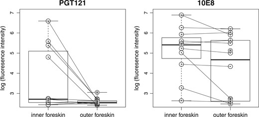
Boxplots of explant infectivity data. Paired observations between inner and outer foreskin samples are connected with lines. Unpaired observations are represented by shaded circles.
5. Discussion
In this article, we investigate how to make more-efficient use of partially paired data in the two-sample comparison problem. Among the many proposals we have studied, we recommend SR-MW|$_{0}^{l}$| and MW-MW|$_{0}^{l}$|. Both are linear combinations of comparison between paired data |$\left\{ \mathcal{X},\mathcal{Y}\right\} $| and comparisons between unpaired data |$\left\{\mathcal{X}^{\prime},\mathcal{Y}\right\} $|, |$\left\{ \mathcal{X},\mathcal{Y}^{\prime}\right\} $|, and |$\left\{ \mathcal{X}^{\prime},\mathcal{Y}^{\prime}\right\} $|, using weights inversely proportional to the variance of each statistic. The difference between SR-MW|$_{0}^{l}$| and MW-MW|$_{0}^{l}$| lies in the choice of test statistic used to compare paired data: SR-MW|$_{0}^{l}$| uses the Wilcoxon signed rank statistic, while MW-MW|$_{0}^{l}$| uses a WMW-type statistic that is equivalent to the linear rank statistics studied in Munzel (1999). This difference has two ramifications: (i) MW-MW|$_{0}^{l}$| may experience slightly elevated type 1 error rates under small sample sizes (e.g. 0.06 when the nominal rate is 0.05), while SR-MW|$_{0}^{l}$| does not; and (ii) MW-MW|$_{0}^{l}$| may be more powerful than SR-MW|$_{0}^{l}$| when the correlation between the two samples is low, e.g. under bivariate lognormal distributions. The proposed methods have been implemented in the R package robustrank, which is available from the Comprehensive R Archive Network.
Our asymptotic results assume that the ratio between the number of missing values and the sample size stays constant. This reflects the reality that in some applications substantial missingness exists due to the inherent challenges in the data collection process. For other applications missingness may be sporadic and the number of missing values may be small. In that case, it is not always better to use combined tests. Limited Monte Carlo studies suggest that the size of the proposed tests, SR-MW|$_{0}^{l}$| and MW-MW|$_{0}^{l}$|, is well controlled and not overly conservative in that scenario (Table D.6 of the supplementary material available at Biostatistics online). The power study (Table D.7 of the supplementary material available at Biostatistics online) suggests that the proposed tests still outperform existing combination tests, but the Wilcoxon signed rank test is more powerful than SR-MW|$_{0}^{l}$|. MW-MW|$_{0}^{l}$| underperforms the Wilcoxon signed rank test for some distributions but outperforms for others. A more thorough investigation into how to choose the best method in practice deserves further investigation.
Although we focus on testing the null hypothesis that the distributions of the two samples are identical, the subset of the proposed methods that are based on the more general variance formulae derived not under the assumption that |$F=G$| may also be applied to test the null hypothesis that relative marginal effect |$\theta$| equals 1/2. One potential obstacle in doing so is the inflated type 1 error rates seen on the right-hand side in Table 1, which occurs because the complexity of the variance formulae requires bigger sample size to justify large sample approximation. An alternative method for ascertaining test significance is by permutation (Pesarin and Salmaso, 2010). For partially paired data, there appears to be no obvious way to perform a permutation-based test, unless one is limited to comparing |$\mathcal{X}$| with |$\mathcal{Y}$| and |$\mathcal{X}^{\prime}$| with |$\mathcal{Y}^{\prime}$|. It is an interesting open question whether it is possible to construct a permutation-based test for partially paired data that makes comparison between all |$X$|’s and all |$Y$|’s.
Our proposed methods use all available data and are valid under the assumption that the missing data mechanism is MCAR. Weaker missing data assumptions have been considered by Akritas and others (2002), Akritas and others (2006), and Gao (2007). An interesting future research direction is to extend these methods so that they also work when the missingness is missing at random (MAR).
Supplementary material
Supplementary material is available at http://biostatistics.oxfordjournals.org.
Acknowledgements
Conflict of Interest: None declared.
Funding
National Institutes of Health [R01-AI122991; R01-GM106177; UM1-AI068635; UM1-AI068618] and the Bill and Melinda Gates Foundation [OPP1099507].
