


Summary
Hamiltonian Monte Carlo has emerged as a standard tool for posterior computation. In this article we present an extension that can efficiently explore target distributions with discontinuous densities. Our extension in particular enables efficient sampling from ordinal parameters through the embedding of probability mass functions into continuous spaces. We motivate our approach through a theory of discontinuous Hamiltonian dynamics and develop a corresponding numerical solver. The proposed solver is the first of its kind, with a remarkable ability to exactly preserve the Hamiltonian. We apply our algorithm to challenging posterior inference problems to demonstrate its wide applicability and competitive performance.
1. Introduction
Markov chain Monte Carlo is routinely used to generate samples from posterior distributions. While specialized algorithms exist for restricted model classes, general-purpose algorithms are often inefficient and scale poorly in the number of parameters. Originally proposed by Duane et al. (1987) and popularized in the statistics community through the works of Neal (1996, 2010), Hamiltonian Monte Carlo promises better scalability (Neal, 2010; Beskos et al., 2013) and has enjoyed wide-ranging successes as one of the most reliable approaches in general settings (Gelman et al., 2013; Kruschke, 2014; Monnahan et al., 2017).
However, a fundamental limitation of Hamiltonian Monte Carlo is the lack of support for discrete parameters (Gelman et al., 2015; Monnahan et al., 2017). The difficulty stems from the fact that the construction of Hamiltonian Monte Carlo proposals relies on a numerical solution of a differential equation. The use of a surrogate differentiable target distribution may be possible in special cases (Zhang et al., 2012), but approximating a discrete parameter of a likelihood by a continuous one is difficult in general (Berger et al., 2012).
This article presents discontinuous Hamiltonian Monte Carlo, an extension that can efficiently explore spaces involving ordinal discrete parameters as well as continuous ones. The algorithm can also handle discontinuities in piecewise smooth posterior densities, which for example arise from models with structural change points (Chib, 1998; Wagner et al., 2002), latent thresholds (Neelon & Dunson, 2004; Nakajima & West, 2013) and pseudolikelihoods (Bissiri et al., 2016).
Discontinuous Hamiltonian Monte Carlo retains the generality that makes Hamiltonian Monte Carlo suitable for automatic posterior inference. For any given target distribution, each iteration only requires evaluations of the density and of the following quantities up to normalizing constants: (i) full conditional densities of discrete parameters, and (ii) either the gradient of the log density with respect to continuous parameters or their individual full conditional densities. Evaluations of full conditionals can be done algorithmically and efficiently through directed acyclic graph frameworks, taking advantage of conditional independence structures (Lunn et al., 2009). Algorithmic evaluation of the gradient is also efficient (Griewank & Walther, 2008) and its implementations are widely available as open-source modules (Carpenter et al., 2015).
In our framework the discrete parameters are first embedded into a continuous space, inducing parameters with piecewise constant densities. A key theoretical insight is that Hamiltonian dynamics with a discontinuous potential energy can be integrated analytically near its discontinuity in a way that exactly preserves the total energy. This fact was realized by Pakman & Paninski (2013) and used to sample from binary distributions through embedding them into a continuous space. This framework was extended by Afshar & Domke (2015) to handle more general discontinuous distributions and then by Dinh et al. (2017) to settings where the parameter space involves phylogenetic trees. All these frameworks, however, run into serious computational issues when dealing with more complex discontinuities and thus fail as general-purpose algorithms.
We introduce novel techniques to obtain a practical sampling algorithm for discrete parameters and, more generally, target distributions with discontinuous densities. In dealing with discontinuous targets, we propose a Laplace distribution for the momentum variable as a more effective alternative to the usual Gaussian distribution. We develop an efficient integrator of the resulting Hamiltonian dynamics by splitting the differential operator into its coordinatewise components.
2. Hamiltonian Monte Carlo for discrete and discontinuous distributions
2.1. Review of Hamiltonian Monte Carlo
Given a parameter |$\theta \sim \pi_{\Theta}(\cdot)$| of interest, Hamiltonian Monte Carlo introduces an auxiliary momentum variable |$p$| and samples from a joint distribution |$\pi(\theta, p) = \pi_{\Theta}(\theta) \pi_P(p)$| for some symmetric distribution |$\pi_P(p) \propto \exp\{- K(p)\}$|. The function |$K(p)$| is referred to as the kinetic energy and |$U(\theta) = - \log \pi_{\Theta}(\theta)$| as the potential energy. The total energy |$H(\theta, p) = U(\theta) + K(p)$| is often called the Hamiltonian. A proposal is generated by simulating trajectories of Hamiltonian dynamics where the evolution of the state |$(\theta, p)$| is governed by Hamilton’s equations:
The next section shows how we can turn the problem of dealing with a discrete parameter |$\theta$| into that of dealing with a discontinuous target density. We then proceed to make sense of the differential equation (1) when |$\pi_{\Theta}(\theta)$|, and hence |$U(\theta)$|, is discontinuous.
2.2. Dealing with discrete parameters via embedding
Let |$N$| denote a discrete parameter with the prior distribution |$\pi_N(\cdot)$|, and assume, without loss of generality, that |$N$| takes positive integer values. For example, the inference goal may be estimation of the population size |$N$| given the observation |$y \, | \, q, N \sim \mathrm{Bi}(q, N)$|. We embed |$N$| into a continuous space by introducing a latent parameter |$\tilde{N}$| whose relationship to |$N$| is defined as
for an increasing sequence of real numbers |$0 = a_1 \leqslant a_2 \leqslant a_3 \leqslant \,{\ldots}\,$|. To match the prior distribution on |$N$|, we define the corresponding prior density on |$\tilde{N}$| as
where the Jacobian-like factor |$(a_{n+1} - a_n)^{-1}$| adjusts for embedding into nonuniform intervals.
Although the choice |$a_n = n$| for all |$n$| is a natural one, a nonuniform embedding is useful in effectively carrying out a parameter transformation of |$N$|. For example, a log-transform |$a_n = \log n$| may be used to avoid a heavy-tailed distribution on |$\tilde{N}$| or to reduce correlation between |$\tilde{N}$| and the rest of the parameters. Mixing of many Markov chain Monte Carlo algorithms, including discontinuous Hamiltonian Monte Carlo, can be substantially improved by such parameter transformations (Roberts & Rosenthal, 2009; Thawornwattana et al., 2018).
While the above strategy can be applied whether or not the discrete parameter values have a natural ordering, embedding the values in an arbitrary order likely induces a multimodal continuous distribution. The mixing rate of discontinuous Hamiltonian Monte Carlo generally suffers from multimodality due to the energy conservation property of the dynamics (Neal, 2010).
2.3. How Hamiltonian Monte Carlo fails on discontinuous target densities
Having recast the discrete parameter problem as a discontinuous one, we focus the rest of our discussion on discontinuous targets. An integrator is an algorithm that numerically approximates an evolution of the exact solution to a differential equation. Hamiltonian Monte Carlo requires reversible and volume-preserving integrators to guarantee symmetry of its proposal distributions; see § 4.1 and Neal (2010). These proposals are generated as follows:
(i) Sample the momentum from its marginal distribution |$p \sim \pi_P(\cdot)$|.
(ii) Using a reversible and volume-preserving integrator, approximate |$\{\theta(t), p(t)\}_{t \geqslant 0}$|, the solution of the differential equation (1) with the initial condition |$\{\theta(0), p(0)\} = (\theta, p)$|. Use the approximate solution |$(\theta^*, p^*) \approx \{\theta(\tau), p(\tau)\}$| for some |$\tau > 0$| as a proposal.
The proposal |$(\theta^*, p^*)$| is then accepted with Metropolis probability (Metropolis et al., 1953)
where |$H(\theta, p) = - \log \pi(\theta, p)$| denotes the Hamiltonian. With an accurate integrator, the acceptance probability of |$(\theta^*, p^*)$| can be close to |$1$| because the exact dynamics conserves the energy: |$H\{\theta(t), p(t)\}= H\{\theta(0), p(0)\}$| for all |$t \geqslant 0$|. The integrator of choice for Hamiltonian Monte Carlo is the leapfrog scheme, which approximates the evolution |$\{\theta(t), p(t)\} \to \{\theta(t + \epsilon), p(t + \epsilon)\}$| by the successive updates
When |$\pi_\Theta(\cdot)$| is smooth, approximating the evolution |$\{\theta(0), p(0)\} \to \{\theta(\tau), p(\tau)\}$| with |$L = \lfloor \tau / \epsilon \rfloor$| leapfrog steps results in a global error of order |$O(\epsilon^2)$| so that |$H(\theta^*, p^*) = H(\theta, p) + O(\epsilon^2)$| (Hairer et al., 2006). Hamiltonian Monte Carlo’s high acceptance rates and scaling properties critically depend on this second-order accuracy (Beskos et al., 2013). When |$\pi_\Theta(\cdot)$| has a discontinuity, however, the leapfrog updates in (2) fail to account for the instantaneous change in |$\pi_\Theta(\cdot)$|, incurring an unbounded error that does not decrease even as |$\epsilon \to 0$|; see the Supplementary Material.
2.4. Theory of discontinuous Hamiltonian dynamics
Suppose |$U(\theta)$| is piecewise smooth; that is, the domain has a partition |$\mathbb{R}^d = \cup_k \Omega_k$| such that |$U(\theta)$| is smooth on the interior of |$\Omega_k$| and the boundary |$\partial \Omega_k$| is a |$(d - 1)$|-dimensional piecewise smooth manifold. While the classical definition of the gradient |$\nabla U(\theta)$| makes no sense on a discontinuity set |$\cup_k \partial \Omega_k$|, it can be defined through a notion of distributional derivatives, and the corresponding Hamilton equations (1) can be interpreted as a measure-valued differential inclusion (Stewart, 2000). In this case, a solution is in general nonunique, unlike that of a smooth ordinary differential equation. To find a solution that preserves critical properties of Hamiltonian dynamics, we rely on a so-called selection principle (Ambrosio, 2008) as follows.
Define a sequence of smooth approximations |$U_\delta(\theta)$| of |$U(\theta)$| for |$\delta > 0$| through the convolution |$U_\delta(\theta) := \int U(\eta) \phi_\delta(\theta - \eta) \, \textrm{d} \eta$|, where |$\phi_\delta(\theta) = \delta^{-d} \phi(\delta^{-1} \theta)$| is a compactly supported smooth function with |$\phi \geqslant 0$| and |$\int \phi = 1$|. Now let |$\{\theta_{\delta}(t), p_{\delta}(t)\}_{t \geqslant 0}$| be the solution of Hamilton’s equations with the potential energy |$U_\delta$|. The pointwise limit |$\{\theta(t), p(t)\} = \lim_{\delta \to 0} \{\theta_{\delta}(t), p_{\delta}(t)\}$| can be shown to exist for almost every initial condition on some time interval |$[0, T]$| (Hirsch & Smale, 1974). The collections of the trajectories |$\left\{ \{\theta(t), p(t)\}_{t \geqslant 0} : \{\theta(0), p(0)\} \in \mathbb{R}^d \right\}$| then define the dynamics corresponding to |$U(\theta)$|. This construction provides a rigorous mathematical foundation for the special cases of discontinuous Hamiltonian dynamics derived by Pakman & Paninski (2013) and Afshar & Domke (2015) through physical heuristics.
The behaviour of the limiting dynamics near the discontinuity is deduced as follows. Suppose that the trajectory |$\{\theta(t), p(t)\}$| hits the discontinuity at an event time |$t_e$| and let |$t_e^-$| and |$t_e^+$| denote infinitesimal moments before and after that. At a discontinuity point |$\theta \in \partial \Omega_k$|, we have
where |$\nu(\theta)$| denotes a unit vector orthogonal to |$\partial \Omega_k$|, pointing in the direction of higher potential energy. The relations (3) and |$\textrm{d} p_{\delta} / \textrm{d} t = - \nabla_{\theta} U_\delta$| imply that the only change in |$p(t)$| upon encountering the discontinuity occurs in the direction of |$\nu_e = \nu\{\theta(t_e)\}$|:
for some |$\gamma > 0$|. There are two possible types of change in |$p$| depending on the potential energy difference |$\Delta U_e$| at the discontinuity, which we formally define as
When the momentum does not provide enough kinetic energy to overcome the potential energy increase |$\Delta U_e$|, the trajectory bounces against the plane orthogonal to |$\nu_e$|. Otherwise, the trajectory moves through the discontinuity by transferring kinetic energy to potential energy. Either way, the magnitude of an instantaneous change |$\gamma$| can be determined via the energy conservation law:
Figure 1, which is explained in more detail in § 3, provides a visual illustration of the trajectory behaviour at a discontinuity.

An example trajectory |$\theta(t)$| of discontinuous Hamiltonian dynamics.
3. Integrator for discontinuous dynamics via Laplace momentum
3.1. Limitation of Gaussian momentum-based approaches
Use of non-Gaussian momentums has received limited attention in the Hamiltonian Monte Carlo literature. Correspondingly, the existing discontinuous extensions all rely on Gaussian momentums (Pakman & Paninski, 2013; Afshar & Domke, 2015; Dinh et al., 2017).
In developing a general-purpose algorithm for sampling from discontinuous targets, however, dynamics based on a Gaussian momentum have a serious shortcoming. In order to approximate the dynamics accurately, the integrator must detect every single discontinuity encountered by a trajectory and then compute the potential energy difference each time; see Algorithm S1 in the Supplementary Material. To see why this is a serious problem, consider a discrete parameter |$N \in \mathbb{Z}^+$| with a substantial posterior uncertainty, say |$\textrm{var}(N \, | \, \text{data})^{1/2} \approx 1000$|. We can then expect a Metropolis move like |$N \to N \pm 1000$| to be accepted with a moderate probability, costing only a single likelihood evaluation. On the other hand, if we were to sample a continuously embedded counterpart |$\tilde{N}$| of |$N$| using discontinuous Hamiltonian Monte Carlo with the Gaussian momentum-based Algorithm S1 in the Supplementary Material, a transition of the corresponding magnitude necessarily requires 1000 likelihood evaluations. The algorithm is made practically useless by such a high computational cost for otherwise simple parameter updates.
3.2. Hamiltonian dynamics based on Laplace momentum
The above example exposes a major challenge in turning discontinuous Hamiltonian dynamics into a practical general-purpose sampling algorithm: an integrator must rely only on a small number of target density evaluations to jump through multiple discontinuities while approximately preserving the total energy. We employ a Laplace momentum |$\pi_P(p) \propto \prod_i \exp(- m_i^{-1} | p_i |)$| to provide a solution. While similar distributions have been considered for improving numerical stability of traditional Hamiltonian Monte Carlo (Zhang et al., 2016; Lu et al., 2017; Livingstone et al., 2019), we exploit a unique feature of the Laplace momentum in a fundamentally new way.
Hamilton’s equation under the independent Laplace momentum is given by
where |$\odot$| denotes elementwise multiplication. A key characteristic of the dynamics in (5) is that |${\textrm{d} \theta}/{\textrm{d} t}$| depends only on the signs of the |$p_i$| and not on their magnitudes. In particular, if we know that the |$p_i(t)$| do not change their signs on the time interval |$t \in [\tau, \tau + \epsilon]$|, then we also know that
irrespective of the intermediate values |$U\{\theta(t)\}$| along the trajectory |$\{\theta(t), p(t)\}$| for |$t \in$||$[\tau, \tau + \epsilon]$|. Our integrator critically takes advantage of this property so that it can jump through multiple discontinuities of |$U(\theta)$| in just a single target density evaluation.
3.3. Integrator for Laplace momentum via operator splitting
Operator splitting is a technique to approximate the solution of a differential equation by decomposing it into components, each of which can be solved more easily (McLachlan & Quispel, 2002). More commonly used Hamiltonian splitting methods are special cases (Neal, 2010). A convenient splitting scheme for (5) can be devised by considering the equation for each coordinate |$(\theta_i, p_i)$| while keeping the other parameters |$(\theta_{{-} i}, p_{{-} i})$| fixed:
There are two possible behaviours for the solution |$\{\theta(t), p(t)\}$| of (6) for |$t \in [\tau, \tau + \epsilon]$|, depending on the initial momentum |$p_i(\tau)$|. Let |$\theta^*(t)$| denote a potential path of |$\theta(t)$|:
In the case that the initial momentum is large enough that |$m_i^{-1} \vert p_i(\tau) \vert > U\big\{\theta^*(t) \big\} - U\{{\theta}(\tau)\}$| for all |$t \in [\tau, \tau + \epsilon]$|, we have
Otherwise, the momentum |$p_i$| flips (|$p_i \gets - p_i$|) and the trajectory |$\theta(t)$| reverses its course at the event time |$t_e$| given by
See Fig. 1 for a visual illustration of the trajectory |$\theta(t)$|. The trajectory has enough kinetic energy to move across the first discontinuity by transferring some kinetic energy to potential energy. Across the second discontinuity, however, the trajectory has insufficient kinetic energy to compensate for the potential energy increase and bounces back as a result.
By emulating the behaviour of the solution |$\{\theta(t), p(t)\}$|, we obtain an efficient integrator of the coordinatewise equation (6) as given in Algorithm 1. While the parameter |$\theta$| does not get updated when |$m_i^{-1} | p_i | < \Delta U$|, line 5, the momentum flip |$p_i \gets - p_i$|, line 9, ensures that the next numerical integration step leads the trajectory toward a higher density of |$\pi_\Theta(\theta)$|. This can be viewed as a generalization of the guided random walk idea by Gustafson (1998).
Coordinatewise integrator for dynamics with Laplace momentum.
1 Function CoordIntegrator|$(\theta, p, i, \epsilon)$|:
2 |$\quad \theta^* \gets \theta$|
3 |$\quad \theta^*_i \gets \theta^*_i + \epsilon m_i^{-1} \textrm{sign}(p_i)$|
4 |$\quad \Delta U \gets U(\theta^*) - U(\theta)$|
5 |$\quad$| if |$m_i^{-1} |p_i| > \Delta U$| then
6 |$\quad \quad \quad \theta_i \gets \theta_i^*$|
7 |$\quad \quad \quad p_i \gets p_i - \textrm{sign}(p_i) m_i \Delta U$|
8 |$\quad$| else
9 |$\quad \quad \quad p_i \gets - p_i$|
10 |$\quad$| return |$\theta, \, p$|
The solution of the original unsplit differential equation (5) is approximated by sequentially updating each coordinate of |$(\theta, p)$| with Algorithm 1, as illustrated in Fig. 2. The reversibility of the resulting proposal is guaranteed by randomly permuting the order of the coordinate updates. Alternatively, one can split the operator symmetrically to obtain a reversible integrator (McLachlan & Quispel, 2002). The integrator does not reproduce the exact solution, but nonetheless preserves the Hamiltonian exactly. This remains true with any stepsize |$\epsilon$|, but for good mixing the stepsize needs to be chosen small enough that the condition on line 5 is satisfied with high probability; see the Supplementary Material.
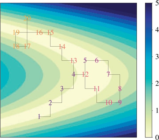
A trajectory of Laplace momentum-based Hamiltonian dynamics |$\{\theta_1(t), \theta_2(t)\}$| approximated by the coordinatewise integrator of Algorithm 1. The log density of the target distribution changes in increments of |$0.5$| and has ‘banana-shaped’ contours. Each numerical integration step consists of the coordinatewise update along the horizontal axis followed by that along the vertical axis. The order of the coordinate updates is randomized at the beginning of numerical integration to ensure reversibility. The trajectory initially travels in the direction of the initial momentum, a process marked by the numbers 1–5. At the fifth numerical integration step, however, the trajectory does not have sufficient kinetic energy to take a step upward and hence flips the momentum downward. Such momentum flips also occur at the eighth and ninth numerical integration steps, again changing the direction of the trajectory. The rest of the trajectory follows the same pattern.
3.4. Mixing momentum distributions for continuous and discrete parameters
The potential energy |$U(\theta)$| is a smooth function of |$\theta_i$| if both the prior and likelihood depend smoothly on |$\theta_i$|. The coordinatewise update of Algorithm 1 leads to a valid proposal mechanism whether or not |$U(\theta)$| has discontinuities along |$\theta_i$|. If |$U(\theta)$| varies smoothly along some coordinates of |$\theta$|, however, we can devise an integrator that takes advantage of the smooth dependence.
We first write |$\theta = (\theta_I, \theta_J)$|, where the collections of indices |$I$| and |$J$| are defined as
More precisely, we assume that the parameter space has a partition |$\mathbb{R}^{|I|} \times \mathbb{R}^{|J|} = \cup_k \mathbb{R}^{|I|} \times \Omega_k$| such that |$U(\theta)$| is smooth on |$\mathbb{R}^{|I|} \times \Omega_k$| for each |$k$|. We write |$p = (p_I, p_J)$| correspondingly and define the distribution of |$p$| as a product of Gaussian and Laplace so that
where |$M_I$| and |$M_J = \textrm{diag}(m_J)$| are mass matrices (Neal, 2010). With a slight abuse of terminology, we will refer to |$(\theta_J, p_J)$| as discontinuous parameters.
When mixing Gaussian and Laplace momenta, we approximate the dynamics via an integrator based again on operator splitting; we update the smooth parameter |$(\theta_I, p_I)$| first, then the discontinuous parameter |$(\theta_J, p_J)$|, followed by another update of |$(\theta_I, p_I)$|. The discontinuous parameters are updated coordinatewise as described in § 3.3. The update of |$(\theta_I, p_I)$| is based on a decomposition familiar from the leapfrog scheme:
Algorithm 2 describes the integrator with all the ingredients put together. When mixing in Gaussian momentum, the integrator continues to preserve the Hamiltonian accurately, if not exactly, with a global error rate of |$O(\epsilon^2)$|; see the Supplementary Material. The advantages of separately treating continuous and discontinuous parameters in this manner are discussed in the Supplementary Material.
Integrator for discontinuous Hamiltonian Monte Carlo.
Function DiscIntegrator|$\left\{\theta, p, \epsilon, \varphi = \texttt{Permute}(J)\right\}$|:
|$\quad p_I \gets p_I + \dfrac{\epsilon}{2} \nabla_{\theta_I} \log \pi(\theta)$|
|$\quad \theta_I \gets \theta_I + \dfrac{\epsilon}{2} \, M_I^{-1} p_I $|
|$\quad$|for |$j \ \mathrm{in} \ J$| do
|$\quad \quad \theta, \, p \gets \texttt{CoordIntegrator}\{\theta, p, \varphi(j), \epsilon\}$|// Update discontinuous params
|$\quad \theta_I \gets \theta_I + \dfrac{\epsilon}{2} \, M_I^{-1} p_I $|
|$\quad p_I \gets p_I + \dfrac{\epsilon}{2} \nabla_{\theta_I} \log \pi(\theta)$|
|$\quad$|return |$\theta, \, p$|
4. Theoretical properties of discontinuous Hamiltonian Monte Carlo
4.1. Reversibility of the discontinuous Hamiltonian Monte Carlo transition kernel
As for existing Hamiltonian Monte Carlo variants, the reversibility of discontinuous Hamiltonian Monte Carlo is a direct consequence of the reversibility and volume-preserving property of our integrator in Algorithm 2 (Neal, 2010; Fang et al., 2014). We thus focus on establishing these properties of our integrator. Let |$\Psi$| denote a bijective map on the space |$(\theta, p)$| corresponding to the approximation of discontinuous Hamiltonian dynamics through multiple numerical integration steps. An integrator is reversible if |$\Psi$| satisfies
where |$R: (\theta, p) \to (\theta, - p)$| is the momentum flip operator. Due to the updates of discrete parameters in a random order, the map |$\Psi$| induced by our integrator is nondeterministic. Consequently, our integrator has the unconventional feature of being reversible in distribution only, |$(R \circ \Psi)^{-1} \overset{d}{=} R \circ \Psi$|, which is sufficient for the resulting Markov chain to be reversible.
For a piecewise smooth potential energy |$U(\theta)$|, the coordinatewise integrator of Algorithm 1 is volume preserving and reversible for any coordinate index |$i$| except on a set of Lebesgue measure zero. Moreover, updating multiple coordinates with the integrator in a random order |$\varphi(1), \ldots, \varphi(d)$| is again reversible in distribution provided that the random permutation |$\varphi$| satisfies |$\left\{\varphi(1), \varphi(2), \ldots, \varphi(d)\right\} \overset{d}{=} \{\varphi(d), \varphi(d - 1), \ldots, \varphi(1)\}$|.
For a piecewise smooth potential energy |$U(\theta)$|, the integrator of Algorithm 2 is volume preserving and reversible except on a set of Lebesgue measure zero.
The proofs are in the Supplementary Material, where we also establish the reversibility and volume-preserving property of discontinuous Hamiltonian dynamics under alternative kinetic energies.
4.2. Irreducibility via randomized stepsize
Reducible behaviours in Hamiltonian Monte Carlo are rarely observed in practice, despite the subtleties in theoretical analysis (Livingstone et al., 2018; Bou-Rabee & Sanz-Serna, 2017; Durmus et al., 2019). However, care needs to be taken when applying the coordinatewise integrator for discontinuous Hamiltonian Monte Carlo; its use with a fixed stepsize |$\epsilon$| results in a reducible Markov chain which is not ergodic. To see the issue, consider the transition probability of multiple iterations of discontinuous Hamiltonian Monte Carlo based on the integrator of Algorithm 2. Given the initial state |$\theta_0$|, the integrator of Algorithm 1 moves the |$i$|th coordinate of |$\theta$| only by the distance |$\pm \epsilon m_i^{-1}$| regardless of the values of the momentum variable. The transition probability in the |$\theta$|-space with |$p$| marginalized out, therefore, is supported on a grid
where |$\theta_J$| as in (7) denotes the coordinates of |$\theta$| with discontinuous conditionals.
This pathological behaviour can be avoided by randomizing the stepsize at each iteration, say |$\epsilon \sim \textrm{Un}(\epsilon_{\min}, \epsilon_{\max})$|. Randomizing the stepsize additionally addresses the possibility that smaller stepsizes are required in some regions of the parameter space (Neal, 2010). While the coordinatewise integrator does not suffer from the stability issue of the leapfrog scheme, the quantity |$\epsilon m_i^{-1}$| nonetheless needs to match the length scale of |$\theta_i$|; see the Supplementary Material for more details.
4.3. Metropolis-within-Gibbs with momentum as a special case
Consider a version of discontinuous Hamiltonian Monte Carlo in which all the parameters are updated with the coordinatewise integrator of Algorithm 1; in other words, the integrator of Algorithm 2 is applied with |$J = \{1, \ldots, d\}$| and an empty indexing set |$I$|. This version is a generalization of random-scan Metropolis-within-Gibbs, also known as one-variable-at-a-time Metropolis. We therefore refer to this version as Metropolis-within-Gibbs with momentum.
We use |$\pi_{\mathcal{E}}(\cdot)$| and |$\pi_{\Phi}(\cdot)$| to denote the distribution of stepsize |$\epsilon$| and of a permutation |$\varphi$| of |$\{1, \ldots, d\}$|, where |$\pi_{\Phi}(\cdot)$| satisfies |$\left\{\varphi(1), \ldots, \varphi(d)\right\} \overset{d}{=} \{\varphi(d), \ldots, \varphi(1)\}$|. With these notations, each iteration of Metropolis-within-Gibbs with momentum can be expressed as follows:
(i) Draw |$\epsilon \sim \pi_{\mathcal{E}}(\cdot)$|, |$\varphi \sim \pi_{\Phi}(\cdot)$| and |$p_j \sim \textrm{Laplace}(\textrm{scale} = m_j)$| for |$j = 1, \ldots, d$|.
(ii) Repeat for |$L$| times a sequential update of the coordinate |$(\theta_j, p_j)$| for |$j = \varphi(1), \ldots, \varphi(d)$| via Algorithm 1 with stepsize |$\epsilon$|.
In this version of discontinuous Hamiltonian Monte Carlo the integrator exactly preserves the Hamiltonian, and the acceptance-rejection step can be omitted.
When |$L = 1$|, the above algorithm recovers random-scan Metropolis-within-Gibbs. This can be seen by realizing that lines 5–9 of Algorithm 1 coincide with the standard Metropolis acceptance-rejection procedure for |$\theta_j$|. More precisely, the coordinatewise integrator updates |$\theta_j$| to |$\theta_j + \epsilon m_j^{-1} \textrm{sign}(p_j)$| only if
where the last distributional equality follows from the fact that |$m_j^{-1} |p_j| \overset{d}{=} \textrm{Ex}(1)$|. To summarize, when taking only one numerical integration step, the version of discontinuous Hamiltonian Monte Carlo considered here coincides with Metropolis-within-Gibbs with a random scan order |$\varphi \sim \pi_\Phi(\cdot)$| and a symmetric proposal |$\theta_j \pm \epsilon m_j^{-1}$| for each parameter with |$\epsilon \sim \pi_{\mathcal{E}}(\cdot)$|. We could also consider a version of discontinuous Hamiltonian Monte Carlo with a fixed stepsize |$\epsilon=1$|, but with a mass matrix randomized |$(m_1^{-1}, \ldots, m_d^{-1}) \sim \pi_{M^{-1}}(\cdot)$| before each numerical integration step; this version would correspond to a more standard Metropolis-within-Gibbs with independent univariate proposals.
Being a generalization of Metropolis-within-Gibbs, discontinuous Hamiltonian Monte Carlo is guaranteed superior performance:
Under any efficiency metric, which may account for computational costs per iteration, an optimally tuned discontinuous Hamiltonian Monte Carlo is guaranteed to outperform a class of random-scan Metropolis-within-Gibbs samplers as described above.
In particular, an optimally tuned discontinuous Hamiltonian Monte Carlo will inherit the geometric ergodicity of a corresponding Metropolis-within-Gibbs sampler, sufficient conditions for which are investigated in Johnson et al. (2013). In practice, the addition of momentum to Metropolis-within-Gibbs allows for a more efficient update of correlated parameters, as empirically confirmed in the Supplementary Material.
5. Numerical results
5.1. Experimental set-up, benchmarks and efficiency metric
We use two challenging posterior inference problems to demonstrate the efficiency of discontinuous Hamiltonian Monte Carlo as a general-purpose sampler. Additional numerical results in the Supplementary Material further illustrate the breadth of its capability. Code to reproduce the simulation results is available at https://github.com/aki-nishimura/discontinuous-hmc.
Few general and efficient approaches currently exist for sampling from a discrete parameter or a discontinuous target density. For each problem, therefore, we pick a few of the most appropriate general-purpose samplers to benchmark against. Chopin & Ridgway (2017) compared a variety of algorithms on posterior distributions of binary classification problems. One of their conclusions is that while random-walk Metropolis is known to scale poorly in the number of parameters (Roberts et al., 1997), Metropolis with a properly adapted proposal covariance is competitive with alternatives even in a 180-dimensional space. As one of our benchmarks, therefore, we use random-walk Metropolis with proposal covariances proportional to estimated target covariances (Roberts et al., 1997; Haario et al., 2001). When the conditional densities can be evaluated efficiently and no strong dependence exists among the parameters, Metropolis-within-Gibbs with componentwise adaptation can scale better than joint sampling via random-walk Metropolis (Haario et al., 2005). This approach is thus used as another benchmark.
For models with discrete parameters, we also compare with the no-U-turn / Gibbs approach (Salvatier et al., 2016). Conditionally on discrete parameters, continuous parameters are updated by the no-U-turn sampler of Hoffman & Gelman (2014). The standard implementation then updates discrete parameters with univariate Metropolis, but here we implement full conditional univariate updates via manually optimized multinomial samplings. In our examples, these multinomial samplings take little time relative to continuous parameter updates, tilting the comparison in favour of no-U-turn / Gibbs. We use the identity mass matrix for the no-U-turn sampler to make a fair comparison to discontinuous Hamiltonian Monte Carlo with the identity mass.
In all our numerical results, continuous parameters with range constraints are transformed into unconstrained ones to facilitate sampling. More precisely, the constraint |$\theta > 0$| is handled by a log transform |$\theta \to \log \theta$| and |$\theta \in [0, 1]$| by a logit transform |$\theta \to \log \left\{ \theta / (1 - \theta) \right\}$| as done in Stan and PyMC (Salvatier et al., 2016; Stan Development Team, 2016). For each example, the stepsize and path length for discontinuous Hamiltonian Monte Carlo were manually adjusted over short preliminary runs by visually examining trace plots. The stepsize for the continuous parameter updates of no-U-turn / Gibbs was adjusted analogously.
The efficiencies of the algorithms are compared through effective sample sizes (Geyer, 2011). As is commonly done in the Markov chain Monte Carlo literature, we compute the effective sample sizes of the first and second moment estimators for each parameter and report the minimum value across all the parameters. Effective sample sizes are estimated using the method of batch means with 25 batches (Geyer, 2011), averaged over the estimates from 8 independent chains.
5.2. Jolly–Seber model: estimation of unknown open population size and survival rate from multiple capture-recapture data
The Jolly–Seber model and its extensions are widely used in ecology to estimate unknown population sizes along with related parameters of interest (Schwarz & Seber, 1999). The model is motivated by the following experimental design. Individuals from a particular species are captured, marked and released back to the environment. This procedure is repeated over multiple capture occasions. At each occasion, the numbers of marked and unmarked individuals among the captured ones are recorded. Individuals survive from one capture occasion to another with an unknown survival rate. The population is assumed to be open so that individuals may enter, either through birth or immigration, or leave the area under study.
In order to be consistent with the literature on capture-recapture models, the notations within this section will deviate from the rest of the paper. Assuming that data are collected over |$i = 1, \ldots, T$| capture occasions, the unknown parameters are |$\{U_i, p_i\}_{i=1}^{T}$| and |$\{\phi_i\}_{i=1}^{T-1}$|, representing
We assign standard objective priors |$p_i, \phi_i \sim \textrm{Un}(0, 1)$| and |$\pi(U_1) \propto U_1^{-1}$|. The parameters |$U_2, \ldots, U_T$| require a more complex prior elicitation; this is described in § 7 of the Supplementary Material, along with the likelihood function and other details on the Jolly–Seber model.
We take the black-kneed capsid population data from Jolly (1965) as summarized in Seber (1982). The data record the capture-recapture information over |$T = 13$| successive capture occasions, giving rise to a 38-dimensional posterior distribution involving 13 discrete parameters. We use the log-transformed embedding for the discrete parameters |$U_i$|. The proposal covariance for random-walk Metropolis is chosen by precomputing the true posterior covariance with a long adaptive Metropolis chain (Haario et al., 2001) and then scaling it according to Roberts et al. (1997). Discontinuous Hamiltonian Monte Carlo can also take advantage of the posterior covariance information, so we also try using a diagonal mass matrix whose entries are set according to the estimated posterior variance of each parameter; see the Supplementary Material for details. Starting from stationarity, we run |$10^4$| iterations of discontinuous Hamiltonian Monte Carlo and no-U-turn / Gibbs and |$5 \times 10^5$| iterations of Metropolis.
The performance of each algorithm is summarized in Table 1. The table clearly indicates superior performance over no-U-turn / Gibbs and Metropolis with approximately 60 and 7-fold efficiency increase, respectively, when using a diagonal mass matrix. The posterior distribution exhibits high negative correlations between |$U_i$| and |$p_i$|, see Fig. 3a. All the algorithms record the worst effective sample size in |$p_1$|, but the mixing of no-U-turn / Gibbs suffers most as |$U_i$| and |$p_i$| are updated conditionally.
Performance summary of each algorithm on the Jolly–Seber model example. The term |$(\pm \ldots)$| indicates the error estimate, twice the standard deviations, of our effective sample size estimators. The path length is averaged over each iteration
| ESS per 100 samples | ESS per minute | Path length | Iteration time | |
|---|---|---|---|---|
| DHMC (diagonal) | 45.5 (|$\pm$| 5.2) | 424 | 45 | 87.7 |
| DHMC (identity) | 24.1 (|$\pm$| 2.6) | 126 | 77.5 | 157 |
| no-U-turn / Gibbs | 1.04 (|$\pm$| 0.087) | 6.38 | 150 | 133 |
| Metropolis | 0.0714 (|$\pm$| 0.016) | 58.5 | 1 | 1 |
DHMC: discontinuous Hamiltonian Monte Carlo. ESS: effective sample size. Iteration time: the computational time per iteration of each algorithm relative to the fastest one.
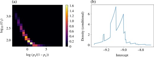
(a) The posterior marginal of |$(p_1, U_1)$| with parameter transformations, estimated from the Monte Carlo samples. (b) The posterior conditional density of the intercept parameter in the generalized Bayes example. The other parameters are fixed at the posterior draw that recorded the highest posterior density among the Monte Carlo samples. The density is not continuous since the loss function is not.
5.3. Generalized Bayesian belief update based on loss functions
Motivated by model misspecification and difficulty in modelling all aspects of a data-generating process, Bissiri et al. (2016) proposed a generalized Bayesian framework which replaces the loglikelihood with a surrogate based on a utility function. Given an additive loss |$\ell(y, \theta)$| for the data |$y$| and parameter of interest |$\theta$|, the prior |$\pi(\theta)$| is updated to obtain the generalized posterior:
While (10) coincides with a pseudolikelihood-type approach, Bissiri et al. (2016) derived the formula as a coherent and optimal update from a decision-theoretic perspective.
Here, we consider a binary classification problem with an error-rate loss:
where |$y_i \in \{-1, 1\}$|, |$x_i$| is a vector of predictors and |$\beta$| is a regression coefficient. The target distribution of the form (10) based on the loss function (11) was suggested as a challenging test case by Chopin & Ridgway (2017). We use the SECOM data from the UCI machine learning repository, which records various sensor data that can be used to predict the production quality of a semiconductor, measured as pass or fail. We first remove the predictors with more than 20 missing cases and then remove the observations that still had missing predictors, leaving 1477 cases with 376 predictors. All the predictors are normalized and the regression coefficients |$\beta_i$| are given |${N}(0, 1)$| priors. Figure 3(b) illustrates the complexity of the target distribution.
In tuning the proposal covariance of Metropolis for this example, adaptive Metropolis performed so poorly that we instead use |$10^5$| iterations of discontinuous Hamiltonian Monte Carlo to estimate the posterior covariance. Scaling the proposal covariance for random-walk Metropolis according to Roberts et al. (1997) resulted in an acceptance probability of less than 0.04, so we scaled the proposal covariance to achieve the acceptance probability of 0.234 with stochastic optimization (Andrieu & Thoms, 2008). We also found the posterior correlation to be very modest in this example, with the ratio of the largest to smallest eigenvalues of the estimated posterior covariance matrix being |$46 \approx 6.8^2$|. This suggested that coordinatewise updates may be competitive, so we implemented Metropolis-within-Gibbs as an additional benchmark. The parameters are updated one at a time with the acceptance rate calibrated around 0.44, as recommended by Gelman et al. (1996). We ran discontinuous Hamiltonian Monte Carlo for |$10^4$| iterations, Metropolis for |$10^7$| iterations, and Metropolis-within-Gibbs for |$5 \times 10^4$| iterations from stationarity.
Table 2 summarizes the performance of each algorithm. Discontinuous Hamiltonian Monte Carlo with identity mass matrix outperforms Metropolis and Metropolis-within-Gibbs by a factor of 330 and 2, respectively. Using a diagonal mass matrix yields only a minor improvement here as the posterior displays similar scales of uncertainty in all the parameters. The mixing of Metropolis suffers substantially from the dimensionality of the target. Conditional updates of Metropolis-within-Gibbs mix well in this example due to weak dependence among the parameters. On the other hand, as demonstrated in the example here and in § 5.2, discontinuous Hamiltonian Monte Carlo not only scales well in the number of parameters, but also efficiently handles distributions with strong correlations.
Performance summary of each algorithm on the generalized Bayesian posterior example. The term |$(\pm \ldots)$| is the error estimate of our effective sample size estimators. The path length is averaged over each iteration
| ESS per 100 samples | ESS per minute | Path length | Iteration time | |
|---|---|---|---|---|
| DHMC (identity) | 26.3 (|$\pm$| 3.2) | 76 | 25 | 972 |
| Metropolis | 0.00809 (|$\pm$| 0.0018) | 0.227 | 1 | 1 |
| Metropolis-within-Gibbs | 0.514 (|$\pm$| 0.039) | 39.8 | 1 | 36.2 |
| ESS per 100 samples | ESS per minute | Path length | Iteration time | |
|---|---|---|---|---|
| DHMC (identity) | 26.3 (|$\pm$| 3.2) | 76 | 25 | 972 |
| Metropolis | 0.00809 (|$\pm$| 0.0018) | 0.227 | 1 | 1 |
| Metropolis-within-Gibbs | 0.514 (|$\pm$| 0.039) | 39.8 | 1 | 36.2 |
DHMC, discontinuous Hamiltonian Monte Carlo; ESS, effective sample size; Iteration time, the computational time per iteration of each algorithm relative to the fastest one.
Acknowledgement
Dunson was supported by the National Science Foundation and Office of Naval Research. Lu was supported by the National Science Foundation.
Supplementary material available at Biometrika online includes the proofs and additional theoretical results on properties of discontinuous Hamiltonian dynamics, the algorithm’s connection to the zig-zag sampler, error analysis of the discontinuous dynamics integrator, as well as additional numerical results.
References
Stan Development Team (
