


Abstract
Data-driven deep learning techniques usually require a large quantity of labeled training data to achieve reliable solutions in bioimage analysis. However, noisy image conditions and high cell density in bacterial biofilm images make 3D cell annotations difficult to obtain. Alternatively, data augmentation via synthetic data generation is attempted, but current methods fail to produce realistic images.
This article presents a bioimage synthesis and assessment workflow with application to augment bacterial biofilm images. 3D cyclic generative adversarial networks (GAN) with unbalanced cycle consistency loss functions are exploited in order to synthesize 3D biofilm images from binary cell labels. Then, a stochastic synthetic dataset quality assessment (SSQA) measure that compares statistical appearance similarity between random patches from random images in two datasets is proposed. Both SSQA scores and other existing image quality measures indicate that the proposed 3D Cyclic GAN, along with the unbalanced loss function, provides a reliably realistic (as measured by mean opinion score) 3D synthetic biofilm image. In 3D cell segmentation experiments, a GAN-augmented training model also presents more realistic signal-to-background intensity ratio and improved cell counting accuracy.
Supplementary data are available at Bioinformatics online.
1 Introduction
Analyzing the single-cell behaviors in the densely-packed bacterial biofilms is key to providing insight for effective treatment of bacterial infectious diseases, such as cystic fibrosis pneumonia (Zhang et al., 2020). However, single-cell analysis in 3D biofilm images remains an open challenge due to densely-packed communities, inhomogeneous intensity and noise (Wang et al., 2017). The advent of deep learning represents an opportunity to solve challenging problems in single-cell analysis. However, such a data-driven approach requires a large quantity of labeled training data to achieve accurate and reliable solutions (Liu et al., 2021b). The current gold standard for labeling biological images is manual annotation, which can be extremely time-consuming and inaccurate, especially for 3D data. The annotation process is inconsistent among different annotators, as fluorescence intensity is often not uniform in cells and cell boundaries are not distinct. It is even more difficult, or nearly impossible, to annotate individual non-spherical cells when densely packed in 3D (Fig. 3, first column), like bacterial cells, for single-cell analysis purpose. Therefore, an automatic ground truth generation method is important for deep learning tasks to obtain a sufficient training dataset.
Data augmentation for microscopy images: For single-cell analysis, major strategies to augment the training dataset before applying deep learning include: (i) performing classic transformations (e.g. scaling, translation, rotation) on limited manually annotated data (Abdollahi et al., 2020; Bloice et al., 2019), which is error-prone to annotated data quality; (ii) simulating the volumes using optical and biological model-based knowledge (Lindén et al., 2016; Zhang et al., 2020) that cannot take into account uncalibrated image aberrations and illumination/emission heterogeneity; and (3) generating synthetic datasets using generative adversarial networks (GAN) (Chen et al., 2021; Dunn et al., 2019). Among all, CycleGAN-based approaches generate images via mapping the distribution between the input and output image domains in a bidirectional manner, which can reproduce realistic scenarios in biomedical datasets (Dimitrakopoulos et al., 2020; Liu et al., 2021a; Sandfort et al., 2019). Most importantly, such a model does not need the input and output images to be structurally aligned to each other, denoted as an unpaired image-to-image translation (Zhu et al., 2017). A successful extension of CycleGAN was tested for a cell label-to-image translation task in Fu et al. (2018), which added spatial consistency loss to reduce the cell location drift in generated images from input binary labels. While works like Fu et al. (2018) and Sandfort et al. (2019) perform training on 2D slices in the 3D images to generate synthetic 3D stacks, they cannot provide sufficient z-axial signal continuity in our bacterial biofilm images. Some works extend the 2D GAN to a 3D GAN (Abramian and Eklund, 2019; Zhang et al., 2018), but they cannot map unmatched labels to images in the training dataset.
Synthetic image quality assessment: The image quality assessment of GAN outputs is another critical step needed to complete the image synthesis work in this project, especially when the output dataset is not structurally aligned with the reference dataset. Image quality assessment assists in selecting a high qualitative synthetic dataset for further deep learning tasks. The regular fully-referenced image quality assessment metrics [e.g. SSIM (Wang et al., 2004)] or comparison-based blind quality assessment methods [e.g. C-IQA (Liang and Weller, 2016)] cannot accommodate our application, because they rely on the overall matching structure and distortion between the ground truth and generated images. The inception score (IS) and the Fréchet inception distance (FID) are more commonly used in evaluating GAN outputs (Heusel et al., 2017; Zhu et al., 2017). However, IS and FID both utilize a pre-trained inception v3 model of 2D images, which cannot directly accommodate 3D dataset evaluation. To automatically assess and learn the conditions in 3D GAN outputs, this article presents a comparison-based stochastic synthetic dataset quality assessment (SSQA) measure that evaluates the relative intensity-wise quality of 2D/3D synthetic dataset compared to the real dataset.
What to expect in this article? This article explores the ideas of unpaired label-to-image translation with CycleGANs (Fu et al., 2018; Zhu et al., 2017), and extends the networks to 3D in order to generate bacterial biofilm image data. Additionally, an unbalanced cycle-consistency loss is presented (Section 2.2) to achieve optimal synthesized biofilm data in 3D when evaluating multiple image quality assessment metrics. Since ground truth annotation is not available in most unpaired image-to-image translation tasks, a stochastic synthetic data quality assessment (SSQA) scheme is also proposed (Section 2.3). Taking the advantage of SSQA and realistic 3D GAN outputs, the biofilm image analysis pipeline can be further improved in terms of higher single-cell counting accuracy and better signal-to-background intensity measure (Section 3.4).
2 Materials and methods
2.1 Training dataset
The 3D biofilm dataset is obtained by way of lattice light-sheet microscopy (LLSM) (Zhang et al., 2020). LLSM is able to look into the dense aggregations of cells in vivo because of its low photo-toxicity and high spatial resolution (Gahlmann and Moerner, 2014). Escherichia coli bacterial cells are used in this article with cytosolic expression of green fluorescent protein. There are 300 3D images with size voxels used for training. These training images contain three time points in biofilm development (Fig. 3, first column). Each image has voxel size of 100 nm nm nm. All the real images are pre-processed with normalization and contrast enhancement that saturates the bottom 1% and the top 1% of all voxel values. The label set contains 300 binary images generated by CellModeller (Rudge et al., 2012) with local densities that approximately match the real image conditions (Fig. 3, second column). For testing, another 300 unseen label images were used to generate synthetic images.
2.2 Biofilm image synthesis with 3D cyclic GAN
2.2.1 3D GAN architecture
The basic framework of the learning module follows the benchmark image synthesis model with CycleGAN (Zhu et al., 2017), which consists of four parts: two generators and two discriminators (Fig. 1). The generators (GLR, GRL) attempt to generate synthetic LLSM images from a binary label set, while discriminators (DL, DR) try to distinguish generated synthetic data from the real data. We adopt the architectures of the downsampling/upsampling style generator with six residual blocks (He et al., 2016) at the bottleneck and patchGANs discriminator with three convolutional layers as used in Fu et al. (2018), which presented promising results in 2D cases. In both networks, we change all the 2D layers to 3D ones. In addition, the original 70 × 70 2D patchGANs discriminator is changed to patch size (depth × height × width) for input of a biofilm image. Replication padding, instance normalization, and the ReLu activation function are used in the generator with employment of the hyperbolic tangent function in the last layer. The discriminator uses LeakyRelu(0.2) and batch normalization. Details about the model parameters of each layer implemented with PyTorch can be found in Supplementary Figure S1.
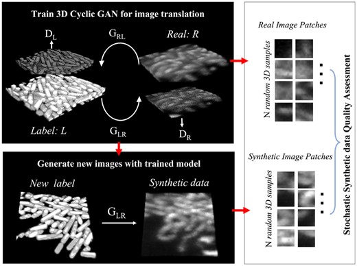
Pipeline for image synthesis and assessment for LLSM 3D bacterial biofilm images. All the images shown are 3D rendered in ImageJ. Step 1: learning the label-to-image translation using 3D cyclic GAN, which contains two generators (GLR, GRL), and two discriminators (DL, DR). Step 2: the learned translation from labels to real images is used to generate synthetic data. Step 3: evaluating the quality of synthetic data with SSQA
2.2.2 Loss function
As the lack of paired data is particularly challenging in our case, and the noise levels and cell sizes differ significantly from those of the original 2D data used in Fu et al. (2018), we investigate different loss functions in the backbone network (CycleGAN) to determine which form provides both the best distribution and spatial consistency for biofilm data. The decision between choosing -norm and -norm in loss functions is always of critical interest. Although -norm is robust for data with outliers, -norm provides unique solutions. Thus, different combinations of p1 and p2 values, including the options listed above, are compared below. We propose an unbalanced cycle-consistency loss, that changing and increasing the weighting of cycle mapping direction by a factor of α = 2 to preserve spatial consistency. In this case, the need for training another network H in 3D will be reduced. Details about the comparison of different loss functions are involved in the next section.
2.3 Synthetic bioimage quality assessment with SSQA
To evaluate the image appearance quality of a generated synthetic dataset compared to the real LLSM biofilm dataset, a Stochastic patch-based Synthetic dataset Quality Assessment (SSQA) method is proposed.
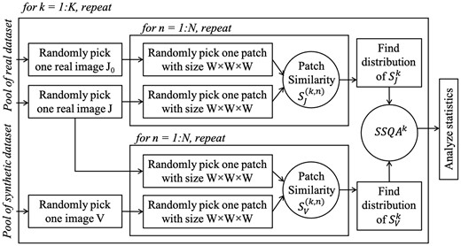
Flowchart to compute and analyze SSQA
Finally, the results of K cross-dataset (real vs. synthetic) SSQA scores are compared graphically in Figure 4. To achieve statistically meaningful SSQA comparisons, an adequate number of stochastic samples are needed in each evaluation based on image size and image numbers in each dataset. In this article, we provide results with samples. Statistical observations (e.g. mean, standard deviation) and intersection-over-union (IoU) of two SSQA histograms are analyzed as listed in Table 1. In terms of a single SSQA, a value closer to zero means better image relative quality. When we evaluate an unpaired dataset containing multiple image conditions, the comparison between intra-dataset (real versus real) and cross-dataset (real versus target) SSQA measures is needed. In this case, a smaller difference between the statistical observations compared to the reference (inter real dataset SSQA0) denotes more similar dataset conditions. The mean values of SSQA, along with standard deviations, are shown in Table 1. The IoU values of SSQAs exhibit quantitative comparison of different synthetic datasets, where a value closer to 1 means the distributions of image intensity-wise qualities in the two datasets are more similar.
Comparison of dataset quality assessment measures (columns) evaluated on different datasets (rows)
| Dataset | MOS | FID | BRISQUE | SBR | SSQA | IoU(SSQA, SSQA0) |
|---|---|---|---|---|---|---|
| Reference | 3.981 ± 1.184 | 1.170e−10 | 36.252 ± 5.997 | 1.767 | 0.026 ± 0.029 | 1 |
| Simulation | – | 122.147 | 41.096 ± 3.269 | 1.567 | 0.019 ± 0.023 | 0.4670 |
| SpCycleGAN | 2.967 ± 1.460 | 45.188 | 34.124 ± 6.796 | 0.926 | 0.030 ± 0.027 | 0.6173 |
| SpCycleGAN 3D | 3.083 ± 1.198 | 103.074 | 38.478 ± 2.187 | 1.234 | 0.018 ± 0.018 | 0.3652 |
| CycleGAN 3D | 3.008 ± 1.345 | 106.938 | 38.092 ± 5.439 | 1.364 | 0.021 ± 0.025 | 0.4371 |
| Ours: 3D Cyclic GAN () | 3.381 ± 1.241 | 80.798 | 34.238 ± 5.155 | 1.418 | 0.028 ± 0.029 | 0.6575 |
Note: FID (Heusel et al., 2017) and BRISQUE are performed on 2D slices in 3D stacks, while the others directly evaluate 3D images. MOS, BRISQUE and SSQA are mean ± standard deviation values. The SBR scores are also averaged over all images in the dataset. Reference denotes the intra-real dataset quality statistics. The closer to the Reference scores, the better relative dataset image quality. The values highlighted in bold are the best results, and the underlined ones in italics are second best.
3 Implementations and discussions
3.1 GAN training and testing
The training of 3D cyclic GAN in this article follows the basic setup in Zhu et al. (2017), which uses Adam optimizer with batch size of one and learning rate of . The learning rate decays linearly after half of the total epochs are completed. Four loss functions are compared: the original SpCycleGAN (Fu et al., 2018), the SpCycleGAN loss function applied in 3D GAN, the original CycleGAN extended to 3D, and the modified unbalanced cycle consistency loss. Other combinations of p1 and p2 values are also tested, but they did not provide reasonable outputs. SpCycleGAN was trained with all the 2D z-sliced images in the 3D stacks, and the other networks are directly trained using 3D cyclic GAN with 300 training data. Each model is trained separately with one NVIDIA Titan v GPU, which takes about a day for training and few minutes for testing. The training time elapse for all the networks follows: SpCycleGAN < 3D Cyclic GAN () < CycleGAN 3D < SpCycleGAN 3D. The testing, or image generation, is performed on another 3D dataset containing 300 images that have never appeared in the training set. Additionally, the model-based simulated dataset and reference real images are shown in Figure 3.
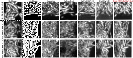
Qualitative comparison of different synthesized results. The images in each column are one slice-view along z-axis in the 3D volume. Real: real enhanced LLSM experimental 3D images, which contain three average biofilm local densities (D), 54.8%, 59.0% and 64.6%, and three signal-to-background ratios (SBR), 2.2, 1.8 and 1.3 (Zhang et al., 2020). Label: label images obtained by CellModeller with comparable local density conditions to the first column. The synthetic outputs for comparison are from model-based simulation (Zhang et al., 2020), original SpCycleGAN (Fu et al., 2018), SpCycleGAN loss in 3D, CycleGAN loss (Zhu et al., 2017) in 3D and our modified 3D cyclic GAN with and in Equation (3). More visual comparisons can be found in Supplementary Figure S2
3.2 Other evaluation metrics
Four other metrics in the literature are evaluated for data quality comparison: human subjective mean opinion score (MOS) for GAN outputs, deep feature-based dataset similarity analysis with FID (Heusel et al., 2017), distortion-based image quality evaluation with BRISQUE (Mittal et al., 2012), and location correspondence evaluation with signal-to-background ratio (SBR) analysis.
Mean opinion score (MOS): The MOS is a reference score that considers human subjective opinion to assess how realistic human observers perceive the GAN output images. Five categories from 1 to 5 are used for the purpose of this article, where each scale denotes one quality level in ‘1—fake’, ‘2—likely to be fake’, ‘3—not sure’, ‘4—likely to be real’ and ‘5—real’. Eighteen participants were each given 100 randomly chosen images from five different datasets. The numbers of images from each set are equal. Each image includes a 2D slice view of the 3D data for evaluation of spatial appearance and a side view examining axial signal continuity. The final score is averaged over the number of participants and the number of data from each dataset. A more realistic dataset will yield a MOS score closer to 5.
Fréchet inception distance (FID): FID score evaluates the quality of GAN outputs based on the statistics from the original real training dataset as well as the statistics in the target outputs (Heusel et al., 2017). It uses a pre-trained inception v3 model to extract deep features that discriminate between real and generated images in terms of mean and covariance. Then, FID calculates the difference of two feature distributions using Fréchet distance. The lower the FID, the better the dataset quality. FID was found to be well-correlated with human judgment, but the inception v3 model was trained on ImageNet 2D images with no 3D interface as of yet. Therefore, only 2D slices in the 3D stacks were evaluated as shown in Table 1.
Blind/referenceless image spatial quality evaluator (BRISQUE): BRISQUE evaluates the distortions in images without the need for corresponding reference images. It measures the deviation of the distributions in normalized distorted images from natural scene images which follow the Gaussian distribution (Mittal et al., 2012). Features in intensity and pixel neighbors are extracted and further analyzed to get a quality score using a support vector regressor. This article uses the original version of BRISQUE, which predicts the distortions in 2D images. For the comparison of dataset quality, a smaller difference of BRISQUE value between the reference and target synthetic dataset is better.
Location correspondence with SBR: The evaluation of location correspondence is performed by overlaying the ground truth labels on generated synthetic data. The values of mean intensity and standard deviation in ‘cell regions’ and ‘background regions’ are extracted. To compare the difference among different datasets, SBR is calculated as described in Zhang et al. (2020) that takes the ratio of foreground to background mean intensities. When the location correspondence is lower, the mean intensity in the foreground gets lower due to the lack of foreground signals, and the mean intensity in the background is higher because of more wrongly-positioned signals. Thus, a higher SBR that is closer to the reference value in Table 1 is better.
3.3 Image quality comparisons
With regard to Table 1, 3D Cyclic GAN () presented the overall optimal dataset quality with the best distortion-based measure (BRISQUE) and best intensity-wise comparisons [SSQA and IoU(SSQA, SSQA0)], corroborated by human subjective MOS. For the other two scores, FID and SBR, 3D Cyclic GAN () still achieves the second-best performance. In visual inspection of different datasets as shown in Figure 3, 3D Cyclic GAN () demonstrates reliable image details that mimic the image conditions in the real dataset. Especially in the background of the images, fewer regions of artifacts or over-smoothness are seen compared to some other synthesized datasets. There are cell drifting problems for all the GAN-generated datasets, but the results of 3D Cyclic GAN () are relatively better.
SpCycleGAN achieved the best FID score and comparable BRISQUE and SSQA scores to 3D Cyclic GAN (), which indicates that the outputs from 2D GAN with the original spatial consistency loss provide decent 2D image intensity-wise and distortion-wise quality conditions. The visual results in Figure 3 also validate the intensity and distortion similarity compared to the real images. SpCycleGAN produces the lowest SBR and MOS, because it cannot preserve the axial signal correspondence along z-axis (Fig. 7) and has more regions of cell signals missing as shown in Figure 3. When this spatial consistency loss is applied in 3D Cyclic GAN, better visual location correspondence, as quantified by SBR, is found in part of the SpCycleGAN 3D outputs, such as the first and last rows in Figure 3. The outputs, however, cannot consistently yield realistic images, where the resultant images are over-smoothed and distorted (see Fig. 3, last row). SpCycleGAN 3D has the lowest mean of SSQA score over all the K image comparisons, but its SSQA frequency does not reflect the similar spread of different image conditions in the real LLSM microscopy image dataset (Fig. 4). Model-based simulation outputs exhibit the best location correspondence in terms of SBR as shown in Figure 7, because the cell signals in the datasets are produced by incorporating the exact locations of cells in labels with theoretical fluorescent emission models, point spread functions, and noise conditions. These simulated datasets are suboptimal, because they cannot mimic the actual intensity and distortion statistics in real datasets with regard to FID, BRISQUE and SSQA.
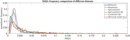
SSQA frequency comparison of different datasets. Histograms of SSQA for all the different outputs are normalized by the total number of K image comparisons to get the frequency of SSQA score in each dataset. The Reference plot indicates the stochastic comparison within the data pool of real images. The more similar the distribution to the Reference, the better relative image quality of the synthetic dataset
In summary, 3D Cyclic GAN () generates the overall most realistic dataset with qualities better than other GAN outputs in terms of intensity, distortion and location correspondence. Additionally, the proposed 3D Cyclic GAN () generated a diverse dataset with a similar mixture of different image conditions as compared to the reference dataset. This diversity in image conditions is observed by the mean and standard deviation values in BRISQUE and SSQA.
3.4 3D Cell segmentation with u-net on real images
After image synthesis, cell segmentation is a key analysis step that can accommodate meaningful cell-level bioinformatics in bacterial biofilm image analysis. In this section, 3D u-net (Çiçek et al., 2016) based experiments are conducted to evaluate the cell segmentation performance involving GAN outputs during the training step.
Training data: The training dataset contains 300 image-and-label sets that include both 3D Cyclic GAN () generated outputs and model-based simulations. The size of each image is , and labels are binary (1 for cell foreground). We argue that combining the two different datasets can reinforce the segmentation model to learn more realistic cell foreground in GAN outputs without losing image-to-label location correspondence provided by simulation. SSQA and SBR metrics are utilized to pick out good quality GAN outputs as substitutions for the corresponding simulated images. In the following segmentation experiments, the top 50 SSQA scores with SBR >1.5 in GAN outputs are selected. Other portions of GAN outputs can be tested based on the generated dataset quality.
Training parameters: A general 3D u-net structure is adopted with three stages of downsampling and upsampling pairs. The kernel size is 33 for both convolution and deconvolution, padded with 1 voxel in all three spatial directions. The stride for convolutions is 2 voxels and 1 voxel for deconvolution operations. Max-pooling with size 23 is used for downsamplers. A residual function of the input at each stage is also learned along the downsampling path for faster convergence (Milletari et al., 2016). Batch normalization and ReLU function are used after convolutions with sigmoid function in the final layer. The number of features for each stage is 64, 256, 256 and 512. A binary cross entropy loss function is chosen in our segmentation task. Batch size, learning rate and the number of epoch are 1, and 200 respectively.
Segmentation performance: For testing, 10 unseen real biofilm images are manually annotated to validate the semantic segmentation accuracy with 3D u-net. Then, we also applied m-LCuts (Wang et al., 2021) to post-process under-segmented u-net outputs to achieve single-cell segmentation. Two single-cell annotated data from Wang et al. (2021) are used for quantitative comparison. By visual inspection, the segmentation outputs from the GAN-involved training model depict more contour details than the simulation-only trained model (Fig. 5).
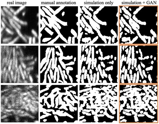
Qualitative comparison of semantic segmentation results using 3D u-net. The images correspond to one slice in the 3D volume. The last column is the segmentation outputs using a combined training dataset involving 3D cyclic GAN () outputs
Quantitatively (see Table 2), although the Dice scores that compare binary segmentation results with manual annotations do not indicate an improvement with the modified training dataset, the margin between the two is not large. One important factor of Dice evaluation comes from the difficulty in accurate manual annotation; cell boundaries can be extremely hard to distinguish in images like row 3 in Figure 5. From a different aspect, with no need for manual annotations, training with GAN outputs can produce SBR scores closer to the reference value (). In addition, the preliminary single-cell segmentation results also show that the GAN-involved training dataset provides better single-cell counting accuracy after m-LCuts (Wang et al., 2021). Cell counting accuracy calculates how many cells can match the ground truth cells if the intersection-over-union (IoU) of the two cell volumes is larger than a thresholding value. For the two images shown in Figure 6, the GAN-involved single-cell segmentation performance is better than the other one for all IoU, ranging from 0.1 to 1. The cell counting accuracy at IoU is shown in Table 2.
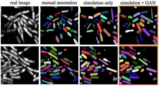
Comparison of segmentation performance with single-cell manual annotation from Wang et al. (2021). The images shown are one slice in the 3D volume
Quantitative comparison of 3D u-net outputs on 10 manually annotated images
| Training data | Dice | SBR | Cell counting accuracy |
|---|---|---|---|
| Simulation only | 0.759 | 1.918 | 56.73%/71.26% |
| Simulation + GAN outputs | 0.750 | 1.779 | 61.73%/76.19% |
| Training data | Dice | SBR | Cell counting accuracy |
|---|---|---|---|
| Simulation only | 0.759 | 1.918 | 56.73%/71.26% |
| Simulation + GAN outputs | 0.750 | 1.779 | 61.73%/76.19% |
Note: Two images that have instance-based manual annotations are evaluated with cell counting accuracy. Bolded values indicate better scores.
Overall, the above 3D cell segmentation performance indicates that the synthetic biofilm dataset generated by 3D Cyclic GAN () can offer an advanced single-cell analysis pipeline for bacterial biofilm images.
3.5 Discussion
The following discussions are to analyze the limitations in the current GAN-based networks for biofilm application, additional model tuning experiments and future directions to improve the GAN outputs for biofilm image studies. Although 3D Cyclic GAN successfully reproduces the real LLSM distributions to generate 3D synthetic datasets, the spatial drifting of each bacterial cell region within the generated images is a limitation of the current GAN-based unpaired biofilm augmentation workflows, as shown in Figure 7. It is worth mentioning that generating a synthetic dataset with unpaired images is challenging in nature, as only about 50% in pixel-wise accuracy was observed in the original unpaired image translation results (Zhu et al., 2017). Additional model tuning experiments aiming to improve the dataset quality in intensity, distortion and spatial consistency were carried out with the presented 3D Cyclic GAN. These efforts include changing the number of layers and parameters in both the generator and discriminator, expanding the training dataset by flipping and cropping, and tuning basic training parameters. For example, we tested learning rate from a scale of to , added and removed up to two layers, and tuned the parameters in the convolutional layers. We also modified the activation layers with a sigmoid function, and varied batch sizes from 1 to 5. None of these trials provided a better synthetic microscopy biofilm output than the current set-up (see Section 2).
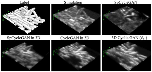
3D comparison of GAN outputs rendered in ImageJ, which shows the preservation of axial (along z-axis) signal continuity with 3D GANs, as well as problems in location drift and missing cells associated with SpCycleGAN (Fu et al., 2018), SpCycleGAN in 3D, CycleGAN (Zhu et al., 2017) in 3D and the proposed 3D cyclic GAN (). The ground truth label volume and model-based simulation result are shown for reference
Taking advantage of the proposed SSQA, improvements in 3D cell segmentation performance are observed when extending the training dataset of u-net with a combination of model-based simulation and filtered 3D Cyclic GAN () outputs. The combined training set strategy aims to maintain high label-to-image structural correspondence as well as fidelity in realistic bioimage appearance. By ranking SSQA scores with the assistance of SBR, the low-quality GAN outputs can be filtered out. Thus, the spatial drifting problem observed in the GAN pipeline is relieved in the application of cell segmentation in bacterial biofilm images. Other future experiments can be explored by adding a small amount of manual annotation of real images to improve the overall GAN location correspondence for the biofilm learning task. Besides, the current biofilm data do not contain enough thick clusters of cells in z-direction that follow the density in CellModeller outputs, so we only selected eight slices of them with a comparable number of cells to label-set images. Collection of more LLSM biofilms data with thicker cluster sizes may be helpful as well.
4 Conclusion
This article explores bioimage synthesis options using GAN to learn and generate densely packed LLSM microscopy 3D biofilm images. A 3D Cyclic GAN with unbalanced cycle consistency loss is presented that can provide the preferable synthetic dataset that mimics the realistic image conditions in the real LLSM dataset, concerning image quality assessment on appearance and distortion conditions. 3D GAN models also ensure axial continuity in signals of cell regions along z-direction when compared to 2D GAN outputs. The proposed stochastic SSQA scheme fills an existing gap in evaluating 3D GAN outputs when the corresponding ground truth images are unavailable. With adequate comparisons in terms of the number of patches and images (e.g. 10 000 × 600 in this article), SSQA reveals meaningful trends of intensity-wise cross-dataset quality. Taking advantage of the presented learning and evaluating pipeline, a GAN-augmented training set can further assist bacterial biofilm image analysis tasks, e.g. 3D cell segmentation. When mixing SSQA-filtered GAN outputs and model-based simulation in training, better single-cell informatics are offered than the simulation-only training process, in terms of more realistic signal-to-background mean intensity ratio and higher cell counting accuracy.
Acknowledgements
We thank Prof. Edward J. Delp and his laboratory at Purdue University for providing the code for DeepSynth (SpCycleGAN).
Funding
This work was supported (in part) by the US National Institute of General Medical Sciences [1R01GM139002 to A.G. and S.T.A.].
Conflict of Interest: none declared.
Data Availability
Software and sample data underlying this article are available in https://github.com/jwang-c/DeepBiofilm.

