Gene regulatory network inference methodology for genomic and transcriptomic data acquired in genetically related heterozygote individuals Free

Abstract

1 Introduction

One of the main goals of Systems Biology is to decipher the complex behaviour of a living cell in its environment. Gene regulatory networks (GRN) are simplified representations of gene-level interactions and network inference methods are powerful tools to reconstruct these networks from observational data (Bellot et al., 2015). Nevertheless, it is often difficult to identify the best-suited method to apply in a specific experimental context. To this end, artificial datasets can be helpful to evaluate different network inference methods and then select the most suitable one to a specific dataset.

1.1 Experimental and biological context

Water deprivation impacts most, if not all cellular and physiological processes during the life cycle of a plant. Numerous studies describing coregulated genes in different organs under different drought scenarios have been reported [reviewed in Shinozaki and Yamaguchi-Shinozaki (2007) and cited more than 2000 times since then]. The inherent complexity resulting from the high number of molecular players as well as the timing and level of their induction into pathways makes molecular deciphering of drought response an archetypal systems biology challenge. Domesticated sunflower (Helianthus annuus) is the major oilseed crop in drought-prone environments in the world because it is considered as tolerant to water deficit (Debaeke et al., 2017; USDA, 2019). (https://www.fas.usda.gov/data/oilseeds-world-markets-and-trade) The production is mainly done by hybrid genotypes to use the heterosis effect. Crossing one female and one male line, the heterosis phenomenon gives progeny more vigorous than either of the two parents (Seiler et al., 2017). Previous works have identified genes controlling drought response in sunflower (Marchand et al., 2014) and these have been shown to be under selective pressure during the breeding of modern hybrids. The responses of sunflower hybrids to drought were shown to be different from those of their parents (Mojayad and Planchon, 1994); for example, the sunflower hybrid species Helianthus  deserticola revealed transgressive gene expression profiles when compared with its parent species H.annuus and Helianthus  petiolaris and this modified response could have been key to its better adaptation to drier environments (Rieseberg et al., 2003; Lai et al., 2006).

1.2 Overview of GNR inference methods

A GRN is an abstract but convenient representation of complex biological processes (Huynh-Thu and Sanguinetti, 2019) and allows representation of direct or indirect regulations between pairs of genes through a simple-directed graph with genes as nodes and pairwise regulations as oriented edges. (We consider here unlabelled edges. Possible labels could have been the regulation sign, activation/repression, its magnitude or a confidence score.) The reconstruction of this graph from observational gene expression data is called the network inference. It is a complex problem with combinatorial [super-exponential number of directed graphs (with $2p(p−1)$ digraphs for p genes, it is larger than the number of atoms in the observable universe for p > 16)] and statistical issues (identifiability and high-dimension). Currently, a number of inference methods, including correlation, regression, mutual information and Bayesian network methods, have been defined. The Dialogue for Reverse Engineering Assessments and Methods (DREAM) challenges resulted in several comparisons of these methods, by providing artificial or experimental datasets (Marbach et al., 2012). Recent reviews on the various network inference methods can be found in Banf and Rhee (2017)), Huynh-Thu and Sanguinetti (2019)) and Saint-Antoine and Singh (2020). In genetical genomics context (Jansen and Nap, 2001), two types of data are available at the same time: (i) expression profiles and (ii) genetic polymorphisms [usually single-nucleotide polymorphisms (SNPs)], for each individual of a population. Then, the combination of these data is exploited by the network inference methods. The DREAM5 Systems Genetics Challenge (https://dreamchallenges.org/dream-5-systems-genetics-challenge) took place in the genetical genomics context by providing challengers datasets composed of gene expression and SNP measurements. A meta-analysis method combining three Bayesian and regression methods was the most successful (Vignes et al., 2011). This meta-analysis method was further improved by including bootstrapping and random forest techniques (Allouche et al., 2013). Other recent approaches have relied on likelihood ratio tests (Wang and Michoel, 2017; Ludl and Michoel, 2021) or a panel of regression and mutual information methods (Zhang et al., 2019) or explored random forest methods with the latter reporting state-of-the-art results on DREAM5 Systems Genetics Challenge (GENIE3) (Huynh-Thu et al., 2013; Huynh-Thu and Geurts, 2019). However, such previous studies in the genetical genomics context have been limited to artificial datasets with a population of independent and homozygous individuals, except for Wang and Michoel (2017); Ludl and Michoel (2021) applied on human and yeast data, respectively.

1.3 Artificial datasets

Different approaches have been tried to design realistic artificial gene expression data (Angelin-Bonnet et al., 2019). SysGenSIM (Pinna et al., 2011) simulates gene expression data from genomic data and artificial networks, SynTReN (Van den Bulcke et al., 2006) exploits real-network topologies from Escherichia  coli or Saccharomyces cerevisiae to simulate gene expression data. Both these approaches rely on deterministic mathematical models of the gene expressions and generate steady-state data using a system of nonlinear ordinary differential equations. Other more complex modelling approaches based on stochastic models, such as GeneNetWeaver (Schaffter et al., 2011), sgnesR (Tripathi et al., 2017) or sismonr (Angelin-Bonnet et al., 2020) produce steady-state or time-series data for mRNA and (complexes of) proteins. sismonr and SysGenSIM are the only simulators to incorporate DNA variation effects in their model. SysGenSIM can produce large steady-state data and was the one used in the DREAM5 Systems Genetics Challenge to produce the artificial datasets.

Identifying the GRN for drought stress response in hybrid sunflower, while being of great interest to both evolutionary biology and plant breeding, constitutes a methodological challenge. In order to choose an efficient network inference method adapted to our biological context, we built artificial datasets with biological properties as close as possible to our experimental dataset. We then applied different network inference methods on the artificial datasets and evaluated their efficiency in our context.

2 Datasets on hybrid genotypes

2.1 Measured dataset

RNA expression data of 173 genes were produced on 353 sunflower hybrids from an incomplete factorial design with 2 × 36 parental lines (Bonnafous et al., 2018) grown under field conditions as described in the data paper (Penouilh-Suzette et al., 2020). Several biological properties are associated with this dataset. First, hybrids are obtained from homozygous parental lines that are genetically connected. Besides, hybrids are heterozygous and gene expressions are subject to heterosis. We selected the measured genes for being mostly transcription factors (TF) annotated for drought sensitivity and responding to it and to heterosis on the data described in Gody et al. (2020) and in the Supplementary Materials (Sections 2 and 3). Expression measurement protocols are fully described in Penouilh-Suzette et al. (2020). SNP markers of the 36 homozygous parental haplotypes were described in Badouin et al. (2017). We deduced the SNPs of the 353 hybrid genotypes by combining those of their two parental haplotypes. The data are available at https://doi.org/10.15454/HESVA0.

2.2 Simulated datasets

To identify the best-suited inference method for our experimental dataset, we needed to construct artificial datasets with biological properties close to the measured one. For this, we designed a three-step strategy: (i) build a reference network, (ii) simulate hybrid genotypes and (iii) simulate gene expression data and adjust parameters.

2.2.1 Build the reference network

We decided to construct an artificial network based on biological information to obtain a realistic shape, particularly in term of graph density heterogeneity. Among plant models, with enough described gene regulations, Arabidopsis  thaliana is the closest to H.annuus. As our measured dataset is composed of a subset of H.annuus genes involved in drought response, we decided to also use a subset of A.thaliana genes to be the nodes of the artificial network. For that, we selected the homologs of our H.annuus genes (Badouin et al., 2017). For 13 pairs of H.annuus genes, the same homolog A.thaliana gene was found. Such A.thaliana genes were duplicated in our artificial network to mimic a recent duplication event as characterized for H.annuus genome (Badouin et al., 2017). Information on gene interactions was sourced from three public databases: (i) AtPID containing interactions between proteins (Lv et al., 2017), (ii) AtRegNet containing regulations between TFs and target genes (Palaniswamy et al., 2006) and (iii) PlantRegMap, including regulations between TFs and other genes (Jin et al., 2017). These databases are compilations of information found in the literature, resulting from experiments or predicted regulations. In these databases, we decided to select only oriented links corresponding to gene regulations (and not protein–protein interactions), involving two genes of our list. Overall, 364 regulations (36 in AtPID, 16 in AtRegNet and 312 in PlantRegMap) were collected to compose our reference network. In the AtRegNet database, the impact on the expression of a target gene is described for some regulations. Among them, 64% induced activation and 36% repression of the expression of the target gene. Hence, for our reference network, we decided to randomly associate a particular type of regulation for each edge with the same probability of activation and repression of expression as in the AtRegNet database. Our chosen reference network consisted of 143 genes distributed into a single connected component of 124 genes and 313 edges with a graph density of 2.1% in addition to 19 unconnected genes (Fig. 1). This graph contains 99 triangles and 7 mutual edge motifs.

Fig. 1.

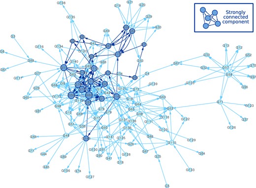
Reference network based on gene–gene interactions from AtPID, AtRegNet and PlantRegMap databases, and composed of 143 genes with 124 genes connected by 313 edges and organized in one component with a density of 2.1%. In this graph, the size of nodes depends on their degree. Dark blue nodes and edges are associated to the same strongly connected component

Open in new tabDownload slide

2.2.2 Simulation of hybrid genotypes

To construct artificial datasets with close biological properties, 463 virtual hybrid genotypes were created from the partial genetic design of 36 × 36 real parents (Bonnafous et al., 2018). To simplify the model of gene regulations used in Section 2.2.3, we considered only one DNA variant per gene based on SNPs present in the genomic and promoter sequence (500 bp. upstream) regions of the gene (Badouin et al., 2017). Using K-medoid clustering with Manhattan distance on the SNP data, for each gene, parental haplotypes were classified into two groups (with a DNA variant score of 0 or 1). The genotype for hybrids on each gene is the sum of the parental scores and can thus be 0, 2 (homozygous) or 1 (heterozygous).

2.2.3 Simulation of gene expressions

To produce simulated measures of expression for the selected genes, we used the SysGenSIM (Pinna et al., 2011) data simulator, based on ordinary differential equations and adapted to the genetical genomics context. In this model, gene expressions are based on the gene network topology and genetic variation (SNP) with only two haplotypes per gene. DNA variants have either a cis-effect (influences the rate of transcription of the gene) or a trans-effect (modifies the efficiency of the gene regulation activity). The equation describing the accumulation of a gene transcript for a given genotype is composed of two parts: the expression of the transcript and its degradation. The expression rate is modulated by the effect of its DNA variant and the expression and DNA variant of the regulators of this gene in the network. Therefore, regulator DNA variants can impact gene regulation and are fed as input data to the simulator. SysGenSIM is designed for homozygous recombinant inbred lines and we slightly modified the simulator to take into account our heterozygous hybrids and mimic allelic dominance, which is important for heterosis. In the case of a heterozygous gene, the DNA variant effect is randomly chosen with an 80% probability to be additive and otherwise (20%) to be dominant for either allele. To generate a simulated dataset in SysGenSIM close to our measured one, we tuned to 25% the cis-to-trans ratio of DNA variant effects to obtain the same heritability (computed as described in Bonnafous et al., 2018) distribution among genes in the two datasets (Supplementary Fig. S1).

By randomly choosing the type of activator or repressor regulations, DNA variant effects (cis or trans) and allelic dominance effects, we successfully produced 100 gene expression datasets. The data are available at https://doi.org/10.15454/vrgwz2. They showed different regulation behaviours for the same reference network and same genotypes (143 genes and 463 hybrid genotypes), that is, they displayed ‘above the best’ or ‘below the worst’ parent heterotic expression. This phenomenon, that represents only a small part of regulatory processes explaining heterosis, was observed in 35 and 41 genes, respectively, suggesting these datasets include larger heterotic expression patterns.

3 Network inference methods

We applied six network inference methods on the simulated datasets to evaluate their accuracy by comparing the inferred networks to the reference network. Four of them were previously applied to the DREAM5 Systems Genetics Challenge (Bayesian Network, Lasso, Random Forest and Findr) (Vignes et al., 2011; Allouche et al., 2013; Huynh-Thu et al., 2013; Wang and Michoel, 2017)) and two are new methods, one based on pairwise exponential Markov random fields (PE-MRF) and the second one exploits genomic relationship between individuals [ordinary least square (OLS) with kinship matrix]. A meta-analysis of the results obtained by these methods was also conducted via the construction of a commensurable score. We present here the specificity and implementation of each method. Given p genes, the expression level of a gene $i∈{1,…,p}$ is noted E_i and $Mi∈{0,1,2}$ represents its haplotypic marker state (in our case it corresponds to the DNA variant score). The methods are used to predict the impact of the expression of a gene E_i on the expression of a gene E_j, $i≠j$ or the impact of the DNA variant M_i on E_j. Further details are given in Supplementary Materials.

3.1 Methods for network inference

Lasso method is used to solve the penalized linear regression problem $Y=Xθ+ε$⁠, where Y is the expression of a target gene E_j and the regressors X are expressions and haplotypic markers of other genes (E_i and M_i), while assuming Gaussian distributions of regressors X and Gaussian noise (ε) (Tibshirani, 1996). We explored an evenly spaced grid of 100 penalization λ values starting from 0 (no penalizations) to a maximum value that prevents a single regressor to be included in any of the regressions (Vignes et al., 2011). We solved the regression problem for each gene expression level E_j with all E_i (⁠$i∈{1,…,p},i≠j$⁠) and haplotypic marker states M_i as regressors, using the least angle regression algorithm implemented in the R glmnet package (Friedman et al., 2010) (https://cran.r-project.org/web/packages/glmnet).

Random forests (Breiman, 2001) are collections of non-linear regression trees $T=(T1,…,TK)$⁠, with $Y=fTk(X)$⁠, partially grown at random using two sources of randomness: (i) each tree is grown using a random bootstrapped-with-replacement sample of the data (having the same sample size) and (ii) the variable used at each split node is selected exclusively from a random subset of all variables (typically of size p/3 for regression). The computation was performed using the randomForest R package (Liaw and Wiener, 2002). For each regression problem (on E_j), the number of trees was set to K = 1000 with other parameters kept at their default value.

Bayesian networks are directed acyclic graphical (DAG) models that capture the joint probability distribution over a set of random variables. All variables (in our case E_i and M_i) are considered as discrete, allowing us to capture non-linear dependencies between variables. For E_i, we used the bootstrapped expression level discretization scheme in at most three values proposed by Vignes et al. (2011). We applied a score-and-search method to find (near) optimal DAGs. BDeu (Heckerman et al., 1995) scores were precomputed using gobnilp. (https://www.cs.york.ac.uk/aig/sw/gobnilp v1.6.3. with a limit of two parents per variable.) The search method combines the local search method MINOBS (Lee and van Beek, 2017), followed by the complete search method elsa (Trösser et al., 2021). [https://gkatsi.github.io/elsa-ijcai21.tar.gz with a CPU time limit of 2 minutes (resp. 20min. for measured data), including 10 s (respectively, 5 min) for MINOBS.] We explored a grid of 50 values for setting the BDeu parameter λ. As in Allouche et al. (2013), constraints were added to forbid edges from expression levels to markers (without biological meaning) and edges between markers (useless information).

PE-MRF (Park et al., 2017) are undirected graphical models recently introduced to model dependencies between different types of data, for example, binary, categorical or continuous data. This model generalizes the graphical Lasso (Friedman et al., 2008) to heterogeneous domains. We applied the PE-MRF approach to the considered dataset with a Gaussian distribution for the node conditional distribution of variables E_i and a categorical distribution for variables M_i. We used a penalization with an $ℓ1/ℓ2$-norm associated with a λ parameter. The values of λ were taken in a log-spaced grid of 100 values from $10−7$ to 10³. These values were chosen to cover the two extreme cases where regulations are predicted between all pairs of genes and where no regulations are predicted at all. Finally, we extract a directed graph from PE-MRF as follows: a predicted undirected edge between two expression levels is transformed into two directed edges and an undirected edge between a marker and an expression level becomes a directed edge from the marker to the expression level.

OLS are simple linear regression methods that minimize the sum of squared errors from the data. Dependencies between hybrids genotypes were taken into account via a relatedness kinship matrix. Edges between expressions and edges from markers to expressions were inferred separately: (i) tests to discover $Mi→Ej$ edges between a target gene expression E_j and haplotypic markers M_i were computed as proposed by Yu et al. (2006) for Genome-Wide Association Studies with no fixed effects; the mean and relatedness kinship matrix were computed as in VanRaden (2008) and (ii) tests to discover $Ei→Ej$ edges were computed as Wald statistics. ASReml-R (Butler et al., 2007) was used to get variance components by restricted maximum likelihood (REML) and to compute Wald statistics.

Findr (Wang and Michoel, 2017) performs multiple likelihood ratio tests for causal inference in the genetical genomic context. We applied it on directed three-variable models involving a pair of gene expressions (E_i, E_j) and the haplotypic marker M_i of the first gene. It assumes gene expressions follow a normal distribution and depend additively on their regulators. It returns an analytical posterior probability $P(Ei→Ej)$ on every directed edge $Ei→Ej, i,j∈{1,…,p}, i≠j$⁠, which is extremely fast to compute. We used the findr R library (pij_gassist function with no diagonal terms).

3.2 Commensurable scores

3.3 Meta-analysis

With S_ij, the meta-analysis score associated with the directed edge from gene i to gene j, and $sijm$ the commensurable score of the edge between i and j obtained by the inference method m, m included in a list of $M$ methods. S_ij varies between 0 and 1. Edges with high scores are those found by most methods to have a high score.

3.4 Selection of the number of directed edges

4 Results

4.1 Network inference on simulated datasets

We applied inference methods described in Section 3 to the 100 simulated datasets of Section 2.2 and compared learnt networks to the reference network.

4.1.1 Efficiency of inference methods

The efficiency of the methods was evaluated using precision and recall (PR) scores. The precision is an indicator of how reliable the predictions are. The recall measures the rate of true edge recovery compared with the full set of true edges. It indicates how comprehensive the predictions are. The PR curves of the six network inference methods and their meta-analysis are shown in Figure 2. We observed that Random Forest dominates the other single methods at the beginning (with recall $<20%$⁠) and then it is overtaken by Findr. For example, at 75% precision, OLS was the less efficient method as only 10.5% of edges of the reference network are found. It is followed by Findr (12.8%), Bayesian Network (15.3%), Lasso (16%), PE-MRF (16.3%) and Random Forest (17.9%). Below this 75% precision level, the slopes of PR curves dropped sharply except for Findr. If we compare the area under PR curves (AUPR score), Findr obtained a better score (0.298) than Random Forest (0.258), the worst being OLS (0.189).

Fig. 2.

PR curves of inference methods on the 100 simulated datasets. Lines represent the median and shaded areas show the 0.25- and 0.75-quantile limits. Dots on the meta-analysis curve correspond to top-k edges for $k∈[50,200]$ and the red dot the graph with minimal density

Open in new tabDownload slide

Meta-analysis over the six methods gave better results than each method alone, as precision of 75% for a recall value of 22.7% is obtained and an AUPR of 0.349.

4.1.2 Selection of the number of edges

We selected the number of edges by applying the approach described in Section 3.4 using a Gaussian kernel with a bandwidth equal to 5. Figure 3 represents the density plots obtained for the 100 datasets. For each value of the network size, we computed the median of the density for the 100 simulated datasets and then smoothed the median curve. The obtained number of edges was 64, corresponding to the smallest density. In the following, we will consider for each simulated dataset, the network built from top-64 edges, where on average graphs had 87.5% precision and 17.89% recall for a density of 1.055%.

Fig. 3.

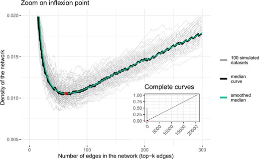
Density of graphs obtained by the meta-analysis, on the 100 simulated datasets, depending on the number of selected edges. The minimal density of the smoothed median (1.055%) is reached for k = 64 edges (red dot, see also Fig. 2)

Open in new tabDownload slide

4.1.3 Description of the meta-analysis network

4.1.3.1 Global network topology

For each of the 100 simulated datasets, a graph was extracted by keeping the top-64 edges. Networks were composed of 79 connected genes on average (from 70 to 86), grouped into 19 components on average (from 13 to 27) per graph. The largest component was composed of 15 genes on average (from 6 to 26).

4.1.3.2 Specific motifs

We examined particular motifs such as triangles and mutual edges that are more likely to be prone to prediction errors. We observed few predicted triangles, between 0 and 6 per graph (2 on average). Among the 191 predicted triangles over the 100 graphs, 2 were correctly predicted, 151 contained an extra edge and 38 had mis-orientated edges. Moreover, the 100 networks contained on average 2 mutual edges (between 0 and 8). In 3% of the graphs, one of the mutual edges was correctly predicted otherwise, an extra edge was inferred by the inference methods.

4.1.3.3 Analysis of errors according to topology

False edges were often located in mutual edges or triangles (47% of errors, Fig. 4A). In the other cases, for each false edge, we investigated the length of the shortest undirected path in the reference network between the two endpoint genes. In total, 33% of remaining errors corresponded to false orientations and 64% to genes that were only connected by a single intermediate gene in the reference network (Fig. 4B).

Fig. 4.

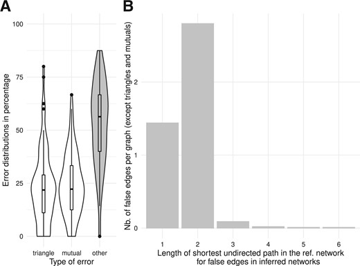
Analysis of error categories based on reference network topology. (A) Distributions of errors according to their location in specific motifs: triangles, mutual edges or other. (B) For other false edges (not included in triangles and mutual edges motifs), distribution of undirected shortest path lengths in the reference network between the genes wrongly connected

Open in new tabDownload slide

4.1.3.4 Node degree

We further compared the out-degree distribution in the reference and inferred networks. Our top-64 edge selection yields sparse graphs with very few large hubs (Fig. 5). In the reference network, we identified a large strongly connected component (23 dark blue nodes in Fig. 1). This relatively dense subgraph containing 70 edges was poorly reconstructed by our approach (with 89.7% precision, but only 11.1% recall on average for the learnt subgraphs induced by the 23 nodes), as shown by the larger difference in out-degree levels between the reference and the inferred networks for those genes (Fig. 5). By selecting genes with a median out-degree greater than 3, $≈19%$ of the top-16 largest hubs in the reference network could be detected in the learnt networks and they do not correspond to the strongly connected component.

Fig. 5.

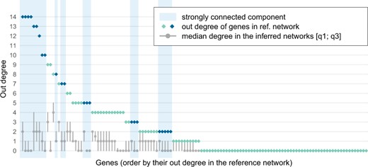
Out-degree levels of genes in the reference network (dark and light blue dots) and networks inferred on the 100 simulated datasets (grey dots). Areas in blue correspond to 23 genes belonging to a large strongly connected component of the reference network

Open in new tabDownload slide

4.2 Network inference on measured dataset

As for networks inferred on simulated datasets, we used the minimal graph density to select 106 top edges corresponding to a graph with minimum density (0.971%) (Supplementary Fig. S2). The inferred network was composed of 105 connected genes grouped in nine components (Fig. 6A). The largest component had 74 genes, only 1 triangle and no mutual edges were predicted. Regarding node connectivity, the out-degree distributions were similar for graphs inferred from simulated and measured datasets as shown in Figure 6B.

Fig. 6.

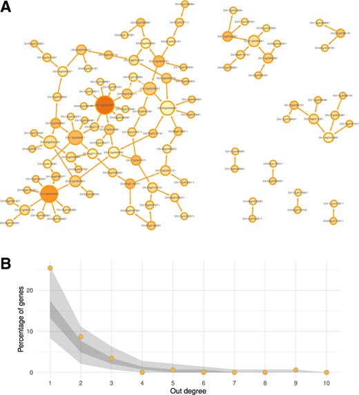
(A) Inferred network on the measured sunflower dataset by the meta-analysis and minimal density selection of 106 edges. Node size depends on its degree and colour to the proportion of out-degree. (B) Comparison of out-degree distributions of genes in the measured network (orange dots) with the 100 networks from simulated datasets. Dark grey area shows the 0.25- and 0.75-quantile limits and light grey area shows extreme values

Open in new tabDownload slide

In this use case, our method identified three hub genes, two regulating five and nine genes and the other one conversely regulated by six genes, an actionable result for biological interpretation.

5 Discussion

5.1 Simulation of gene expression datasets for hybrid genotypes

To simulate more realistic gene expression datasets compatible with the larger genetic variability and heterozygosity observed in wild populations and genetic resources, we improved the SysGenSim simulator at the genetic level. First, since gene expressions are subject to heterosis effects (Lai et al., 2006), we implemented a dominance or additive effect of each allele in the simulator to simulate this phenomenon. Secondly, the different parameters of the simulator were adjusted to have the same heritability in the measured and simulated datasets. Concerning the topology, we note that whole-genome duplications lead to numerous paralog genes such as observed in the sunflower genome (Badouin et al., 2017), which will differentiate and display different expression patterns. To take this into account, we integrated artificial paralogous genes with the same regulators and regulated genes. SysGenSim allowed setting different biological parameters (basal level, regulation strength, etc.) for the two paralogs and can thereby lead to different expression levels, which is in accordance with observed real datasets. Moreover, real networks have a modular structure with some dense component parts and we successfully included this complexity of biological networks in our reference network (e.g. the presence of a large strongly connected component). These improvements allowed us to simulate gene expression datasets with properties very similar to measured ones. In the future, a challenge would be to introduce higher genetic variability, that is, having more than two possible haplotypes per gene.

5.2 Comparison of inference methods

Six different inference methods were tested on simulated datasets, each of them having its own specificity. For example, Findr and PE-MRF could handle together continuous (as expression levels) and discrete (as SNPs) data with different distribution assumptions. Lasso and Random Forest considered both data as continuous whereas Bayesian networks considered them as discrete. All the methods used both data together except for OLS that ran them separately. OLS was the only tested method taking into account the dependencies between genotypes via a kinship matrix. However, results from OLS were inferior possibly due to the lack of bootstraps. As expected, the meta-analysis achieved greater efficiency than each method taken individually. Concerning computation time and resources, Findr, Lasso and Random Forest ran in less than 2 min per simulated dataset on a personal computer. OLS took longer, around 2 h on a server and required commercial software (ASReml). Bayesian networks and PE-MRF were the most demanding approaches taking hours on a 20-CPU Xeon 3 GHz server. The meta-analysis could be run on a personal computer within a few minutes. For cases where computing resources may be limited or the number of genes too high, it could be interesting to consider only the fastest methods for the meta-analysis (Lasso, Random Forest and Findr). For example, on our simulated datasets, the recall for 75% precision was similar: 22.0% with the light meta-analysis, compared with 22.7% with the complete one (Supplementary Fig. S3). We compared our approach with results from previous studies (Allouche et al., 2013; Huynh-Thu et al., 2013; Huynh-Thu and Geurts, 2019; Vignes et al., 2011) using one artificial dataset provided by the DREAM5 Systems Genetics Challenge. This is composed of expression measures for 1000 genes, on 999 individuals with no dependencies among them, a modular scale-free network with 2048 edges (Network1) and homozygous markers. Due to the size of the problem, we applied the light meta-analysis version and found an AUPR score of 0.65 and selected 607 edges with the smallest density criteria (Supplementary Figs S4 and S5). This is clearly superior to another similar meta-analysis approach based on three methods [Bayesian network, Lasso and Dantzig selector (Candes et al., 2007)] that found an AUPR score of 0.482 (Vignes et al., 2011), to Findr 0.547 [Supplementary Table S1 in Wang and Michoel (2017)] and GENIE3-SG-sep(product) 0.58 (Huynh-Thu et al., 2013). On our much smaller but more realistic simulated datasets, we found an AUPR of 0.349 with our complete meta-analysis strategy. Therefore, we believe our simulated datasets constitute a challenging benchmark for the Systems Biology community.

5.3 Characterization of obtained networks

By selecting the minimal density network, inferred networks were always sparse. Thus, the highly connected parts of the network were difficult to identify. Having a sparse graph may be an advantage if we try to identify peripheral genes that can indirectly modulate a target phenotype, for example, the resistance of sunflower to drought in our case, through a chain of regulations towards highly connected key genes (Liu et al., 2019). In addition, by minimizing the density of the network, we performed a very stringent procedure and selected a reduced number of edges but with a higher probability of correctness. With this procedure, we noticed that predicted motifs such as triangles or mutual edges were still prone to errors and represented half of the false edges. Other errors consisted mainly of wrong orientations or were likely due to a missing intermediate gene. Similar results are expected on measured datasets. When analysing and validating a newly inferred network, we recommend the following guidelines: (i) when triangles or mutual edges are predicted, a specific validation step must be included since one edge is probably false; (ii) when an edge is in contradiction with literature, it could be due to an orientation error; (iii) when experimental data cannot validate a direct interaction between the product of a gene and the gene it regulates, it could be due to the lack of an intermediate actor and (iv) interaction between two genes can be experimentally demonstrated even if an edge is not present in the graph since many edges are not predicted.

5.4 Application on a measured dataset

For our measured dataset, the number of genes was slightly higher (173 instead of 143) and the number of measured hybrid genotypes was lower (353 versus 463) than for our simulated datasets. Following our density minimization procedure, we selected 106 edges (only 64 for simulated datasets). This variation of size can be explained by different factors: evolutionary differences between sunflower and model plants used to develop the reference dataset, reduction of genetic diversity and/or modelling hypotheses on allelic and gene expression effects in the simulation model. Importantly, the resulting network serves as a working hypothesis for biologists. For example, one of the major regulatory genes found, HanXRQChr16g0529981, is homologous to the NMD3 gene in the plant model A.thaliana and found more abundant in cold (physiologically related to drought) condition for this plant (Cheong et al., 2021). The most regulated gene found in our network, HanXRQChr02g0058891, is a TF involved in seed oil content in Brassica napus (Rajavel et al., 2021) and shows an interaction with the abiotic stress genes in A.thaliana (Katiyar and Mudgil, 2019). These genes could be good new candidates for future studies on abiotic stress of H.annuus with prior knowledge of molecular and epistatic interactors. Beside the scope of this methodological article, future challenges will consist in increasing the dataset dimensions, that is, more genes, performing a complete functional study including GO analysis, colocalization with drought response controlling QTL (Gosseau et al., 2019) and testing network robustness in the context of heterozygosity.

6 Conclusion

To choose an inference method adapted to our biological context, we created artificial datasets with realistic biological properties. To build such artificial datasets, our approach was carried out in four steps: (i) build a reference network based on available biological information; (ii) create artificial haplotypes based on genomic information available for the hybrid genotypes; (iii) choose and adapt a gene expression simulator and (iv) adjust the simulator parameters based on a comparison of the heritability score obtained on measured and simulated datasets. We believe that this approach can be easily adapted to other biological experiments and genetic data to build artificial datasets with other biological properties. This approach allowed us to choose a meta-analysis strategy based on six inference methods adapted to our datasets that was completed by a novel strategy to select the minimal density network. The resulting learnt networks are very sparse, which should favour precision at the expense of recall and the inherent difficulty to detect large hubs. Therefore, this methodology is directly applicable to other gene expression datasets of similar sizes, combined or not with genotypic information.

Acknowledgements

We are grateful to the staff at GenoToul Bioinformatics (Toulouse, France) and IFB Core (Evry, France) platforms for computational support provided during this work and Revathi Bacsa for editorial assistance.

Funding

This work was supported by the SUNRISE project of the French National Research Agency (ANR-11-BTBR-0005, 2012-2020).

Conflict of Interest: none declared.

References