


Abstract
Precise prediction of cancer subtypes is of significant importance in cancer diagnosis and treatment. Disease etiology is complicated existing at different omics levels; hence integrative analysis provides a very effective way to improve our understanding of cancer.
We propose a novel computational framework, named Deep Subspace Mutual Learning (DSML). DSML has the capability to simultaneously learn the subspace structures in each available omics data and in overall multi-omics data by adopting deep neural networks, which thereby facilitates the subtype’s prediction via clustering on multi-level, single-level and partial-level omics data. Extensive experiments are performed in five different cancers on three levels of omics data from The Cancer Genome Atlas. The experimental analysis demonstrates that DSML delivers comparable or even better results than many state-of-the-art integrative methods.
An implementation and documentation of the DSML is publicly available at https://github.com/polytechnicXTT/Deep-Subspace-Mutual-Learning.git.
1 Introduction
In the past, cancer was considered to be a single type of disease, and diagnosed conventionally via the morphological appearance of tumor. This strategy conducts serious limitations that some tumors share similar histopathological appearance, but they have significant different clinical manifestations and represent different outcome of therapy. Nowadays, increasing evidence from modern transcriptomic studies has supported the assumption that each specific cancer is composed of multiple subtypes, which refers to groups of patients with corresponding biological features or a correlation in a clinical outcome, e.g. response to treatment or survival time (Heiser et al., 2012; Jahid et al., 2014; Prat et al., 2010). The cancer subtypes prediction has been the crux of cancer treatment, since it could induce target-specific therapies for different subtypes and help in providing more efficient treatment and minimizing toxicity on the patients. Furthermore, cancer subtypes prediction may accelerate our understanding of cancer evolution, the advancement of patient stratification and the pace of design new effective therapeutic methods (Alizadeh et al., 2015; Bailey et al., 2016).
Usually, a suitable prediction of any disease has to be scientifically sound, clinically useful, easily applicable and widely reproducible (Viale, 2012). The cancer subtype prediction usually involves two stages: subtypes discovery and subtypes classification (Collisson et al., 2019). The discovery refers to the detection of previously unknown subtypes (Mo et al., 2013). The pattern discovery of cancer subtypes is still a challenging open problem, since different conclusions of cancer subtypes number have been drawn by using different research methodologies and data sources. For instance, glioblastoma multiforme (GBM) is estimated as two subtypes (Nigro et al., 2005), three subtypes (Wang et al., 2014), four subtypes (Sanai, 2010) and six subtypes (Speicher and Pfeifer, 2015) in different works of literature, respectively. In contrast, classification refers to the assignment of specific samples to already-defined subtypes (Bailey et al., 2016). This task can be achieved via supervised learning methodology. The cancer data could be obtained only from a sample with clinical follow-up, which is a laborious and time-consuming procedure. However, supervised learning does not seem to cherish the data, since it only employs labeled data while disregards unlabeled data in training. Whereas, clustering-based methods do not need or have the luxury of known types as training set, thus they are widely used for taking full advantage of unlabeled data (Gao and Church, 2005).
High-throughput experimental technologies have provided a large amount of omics data, which enables the development of analysis genomic patterns of cancers and prediction cancer subtypes at molecular levels. Usually, gene expression alterations regulate the growth and differentiation of cells, which are major components in transforming normal cell to cancer cell (Croce, 2008). As the molecular complexity of cancer etiology exists at all different levels, there have been some attempts at cancer prediction using omics measurements at different levels, including mRNA, miRNA and DNA methylation (Beroukhim et al., 2010; Davis-Dusenbery and Hata, 2010; Lu et al., 2005; Noushmehr et al., 2010; Wood et al., 2007) . The cancer development and progression are influenced by molecular mechanisms spanning through different molecular layers (Chin and Gray, 2008; Hanash, 2004), hence a recent growing trend in cancer subtypes prediction is to integrate individual omics data for capturing the interplay of molecules (Ritchie et al., 2015; Wang et al., 2014). It helps to assess the flow of information from one omics level to the other and to bridge distance from genotype to phenotype. Some large national and international consortia, such as The Cancer Genome Atlas (TCGA) and International Cancer Genome Consortium, have collected abundance of biological samples assaying multi-level molecular profiles. A large amount of data provides more detailed information to characterize different subtypes, and to study the biological phenomenon holistically. Meanwhile, it poses great challenges for integrative analysis (Shen et al., 2009; Zhang et al., 2012).
Many appealing methods of multi-level omics integration have been widely exploited and proposed. Akavia et al. (2010) adopted Bayesian network to identify mutations drivers. Lanckriet et al. (2004) proposed a kernel-based algorithm to integrate heterogeneous descriptions of omics data straightforwardly. Kim et al. (2012) predicted clinical outcomes in brain and ovarian cancers via a graph-based algorithm. Shen et al. (2009) proposed iCluster algorithm to discover potentially novel subtypes via analysis variance–covariance structure. Wang et al. (2014) proposed a network based algorithm, i.e. Similarity Network Fusion (SNF), to aggregate different genomic data types. Liu and Shang (2018) designed a hierarchical fusion framework to use diverse similarity networks generated by multiple random sampling. Nguyen et al. (2017) proposed a radically integrative approach, Perturbation clustering for data INtegration and disease Subtyping (PINS), which constructs connectivity matrices for describing the co-clustering of samples in a same omics level and integrates these matrices. Wu et al. (2015) designed a Low-Rank Approximation based multi-omics data clustering (LRAcluster) model to share principal subspace across multiple data types. Rappoport and Shamir (2019) proposed a NEighborhood based Multi-Omics clustering (NEMO) method, which constructs similarity matrix for each omics level and calculates average similarity matrix for overall omics data.
Most integrative analyses holistically using multiple data levels could be more powerful than individual analyses independently using a single data level. However, that integrative analyses are carried out successfully should be based on the premise that each level data needed for fusion is available and complete. These preconditions restrict the applicability in clinical practice. In modeling prediction, the training data can be obtained from public database resources, which contain various levels of genomic data. Whereas patients who need to be diagnosed might lack some levels of genomic data used in the model training. This fact may lead to the trained holistic model becoming unavailable. From a machine-learning perspective, the integrative analysis corresponds to multi-view learning. Some level data missing can be described as the phenomenon that the number of views in training process is more than the number of views in test process. In order to fully utilize the complementary information contained in the different level omics data, we introduce the mutual learning mechanism (Zhang et al., 2018) for improving the performance not only on integrative analyses, but also on the individual and partial data analyses.
Subspace learning aims at finding out some underlying subspaces to fit different groups of data points, which has attracted considerable attention in computer vision and machine learning (Lerman and Maunu, 2018; Peng et al., 2018, 2020). In biological research field, there have been some attempts using subspace learning to deal with clustering problem (Liu et al., 2018; Zheng et al., 2019). Besides, mutual learning is recently proposed as a novel machine-learning paradigm by constructing a pool of students who simultaneously learn to solve the task together. Specifically, students are trained for a two-part aim: independent learning objective of each student itself and consistent learning objective of all students together. Wu et al. (2019a) proposed a complementary correction network to capture the complementary information to enhance learning performance. Kanaci et al. (2019) proposed a multi-task mutual deep-learning model to learn features simultaneously from different students and to achieve a consensus learning by fuzing features from all students. Wu et al. (2019b) adopted the mutual learning strategy to detect diverse features and fuze intertwined multi-supervision. For multi-level omics data integrative analysis, each student corresponds to the model learnt from each level data. The independent learning objective of each student is to exact discriminative features from given single-level data, while the consistent learning objective of all students is clustering the patients. This paradigm jointly trains multiple model branches specialized for each single omics data and achieves the integration at the same time.
In this article, we propose the Deep Subspace Mutual Learning (DSML) method to capture the subspace structures in each level of omics data and in the entire fuzed data for cancer subtypes prediction. In our integrative method, deep networks are constructed including several branch models and a concentrating model. Firstly, auto-encoder and data self-expressive layers are utilized in each branch model to encode latent feature representations hidden in each level data. Secondly, a concentration model is used to uncover the global subspace structure in entire data. Finally, cancer subtypes are predicted by spectral clustering based on the obtained global subspace structure. A joint optimization problem supporting mutual learning is proposed to achieve balanced emphases on each branch and consensus losses. To our best knowledge, it is the first attempt at using mutual learning in unsupervised scenario and bioinformatics field. In addition, there have been no previous works simultaneously to enhance the prediction performance on multi-level omics cancer data and single omics cancer data.
The experiments conducted on five public cancer datasets demonstrate that DSML generally delivers comparable or even better clustering results than other state-of-the-art algorithms. That is, DSML can discover meaningful cancer subtypes from multi-level omics data, meanwhile provide a prospective avenue for understanding cancer pathogenesis and promoting personalized cancer treatment.
2 Materials and methods
DSML is mainly composed of calculating data representation via DSML model and predicting cancer subtypes via spectral clustering algorithm. We describe the details of each step in the following.
2.1 Data representation
2.1.1 Single-level omics data representation learning model
Conventional data representation techniques try to find a lower-dimensional subspace for best fitting a collection of points sampled from a high-dimensional space, which assumes that the data are drawn from a single subspace. But in practice, much high-dimensional data should often be modeled as samples drawn from the union of multiple subspaces. Subspace clustering (Soltanolkotabi et al., 2013; Wang and Xu, 2016) refers to the task of uncovering the underlying structure of data and clustering the data into their inherent multiple subspaces. The mainstream strategy of subspace clustering is to represent each data point by a linear or affine combination of remaining data points with sparse constraints, i.e. data linear self-expressiveness (Elhamifar and Vidal, 2013).
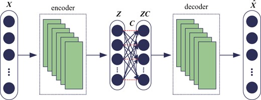
Structure of DSCN
The stacked convolutional auto-encoder (Du et al., 2017; Masci et al., 2011) structures are selected for reflecting the interactions between genes indirectly. The Rectified Linear Unit (Krizhevsky et al., 2012) is adopted as non-linear activation function in convolutional layers. The nodes in self-expressive layer are connected fully by linear weights, i.e. C, without bias and non-linear activations. The input data of self-expressive layer is the output of the encoder layers involving non-linear activation function. Hence, although only linear connections are used in self-expressive layer, the whole networks will still achieve the non-linear self-expressive of data. The weight between two corresponding points in self-expressive layer should be set to zero, i.e. constraint in Equations (4) and (5), denoted as red dashed lines in Figure 1.
2.1.2 Multi-level omics data representation learning model
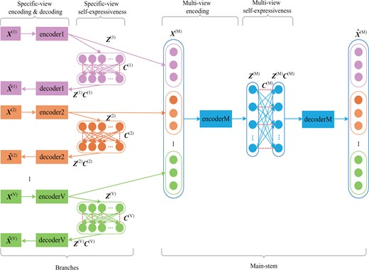
Overview of DSML. DSML is composed of several branches (pink, orange and green standing for different views) to achieve specific-view encoding and specific-view self-expressiveness, and a concentrated main-stem (shown with blue) to realize multi-view encoding and multi-view self-expressiveness. Specific-view encoding extracts latent feature representations automatically from each view and specific-view self-expressiveness uncovers the intra-view similarity. Accordingly, the holistic representations from different views are connected and integrated via multi-view encoding. The holistic similarity leant from multi-view self-expressiveness could be used for subsequent clustering task
Each notation in Equation (6) has a similar meaning to Equation (5). However, in the context of multi-view, V denotes the branches for V individual level omics data and M denotes the main-stem for integrated data. That is, , where is output of encoder in vth branch, i.e. the extracted feature of vth level omics data. The notation T denotes the transpose of a vector or a matrix.
The networks with the structure of branches and main-stem incorporating joint optimization in its design can realize mutual learning. The branches can be seen as the students’ pool. The independent learning aim of each branch is to obtain the individual representation and similarity in each omics data, while consistent learning aim of main-stem is to get the similarity in overall level omics data. DSML is a kind of feed forward neural networks, hence the representation of each omics data, i.e. , can effect on the connection weights within main-stem part. DSML is optimized through back propagation strategy, hence the learning of main-stem part in turn effects on the of each branch. Furthermore, the representation also influences on the similarity relationship, i.e. self-expressive weights . Eventually, the mutual learning is carried out among specific-view encoding and self-expressiveness as well as multi-view encoding and self-expressiveness. Consequently, all of them will be improved in training process. Besides, each branch in trained DSML can be employed as an independent model for uncovering the representation and similarity on single-level data. Since multi-level omics data are involved in training, each trained branch has contained the complementary information from other level data. In practice, even if the patients only have one level of data in test, the prediction made by trained branches can also achieve satisfactory results.
The DSML training algorithm.
Input: Multi-level data , trade-off parameters and .
Output: Self-expressive weights .
1: Construct and train auto-encoder networks for vth level data by minimizing reconstruction error .
2: Initialize specific-view encoding and decoding parts with for each level data.
3: Learn specific-view self-expressive weights and fine-tune all branches by Equation (5).
4: Connect representation from each branch to form input data of main-stem part.
5: Construct and train auto-encoder networks by minimizing reconstruction error .
6: Initialize multi-view encoding and decoding with .
7: Learn and fine-tune self-expressive weights in main-stem by Equation (5).
8: Fine-tune overall DSML networks by Equation (6).
9: return
2.1.3 DSML for partial-level omics data
DSML incorporates the mutual learning mechanism, such that it can handle datasets where only a subset of the omics was measured for some samples, i.e. partial-level omics data. As shown in Figure 2, each branch aims to learn the representation and similarity of data from each omics level, and the main-stem controls the consensus learning by fuzing representation from all branches. Consequently, each branch can be seen as an independence model to deal with single omics level data. In clinical applications, even though the patient who needs to be diagnosed only has single omics level data, the corresponding branch within DSML could still achieve satisfactory prediction results, since this branch model has already involved information from other omics in training stage via mutual learning. Moreover, if the data of ith patient has several omics but lost vth omics, we could set equals to the all-zero vector and input it directly to the complete DSML model. This lost omics data would not produce a noticeable effect on the representation of overall data fusion. DSML thereby automatically omits the lost omics data and utilizes the available partial-level omics data to predict the cancer subtypes in a natural manner.
2.2 Spectral clustering
2.3 Materials
In this article, five publicly available benchmark datasets from TCGA have been used to validate the ability of different integrative algorithms. These datasets are for the following cancer types: Breast Invasive Carcinoma (BIC), COlon ADenocarcinoma (COAD), GBM, Kidney Renal Clear Cell Carcinoma (KRCCC) and Lung Squamous Cell Carcinoma (LSCC). Three levels omics data: mRNA expression, miRNA expression and DNA methylation are used for analysis each cancer type. All datasets used in this article preprocessed as in Rappoport and Shamir (2018, 2019). The corresponding codes can be downloaded from the NEMO website (http://acgt.cs.tau.ac.il/nemo/). The number of patients ranges from 184 for KRCCC to 621 for BIC.
3 Results
The proposed method DSML is compared to six multi-omics prediction algorithms on five full multi-level cancer datasets, and then compared to some methods on these cancer datasets with partial level of data.
3.1 Full multi-level omics datasets
Several experiments were performed to demonstrate the effectiveness of multi-level omics data integrating and clustering for cancer subtypes prediction. We compare our DSML on each dataset to six different methods. We select the classical method SNF, as well as other relevant approaches, including Consensus Cluster (CC) and SNF.CC, which are implemented via R packages Cancer Subtypes (Xu et al., 2017). Moreover, we adopt some late integrative methods, such as PINS, LRAcluster and NEMO.
The survival curves of different clusters and performed enrichment analysis on clinical labels are selected to assess the clustering performance (Rappoport and Shamir, 2019). The P-value is adopted for survival analysis. The logrank test of the Cox regression (Hosmer and Lemeshow, 1999) model is used, in order to assess the significance of the difference in survival profiles between subtypes. The P-value represents that the observed difference in survival is characterized by the possibility of accidental discovery. For enrichment analysis, the same set of clinical information is adopted for all cancers, including age at initial diagnosis, gender as well as four discrete clinical pathological parameters, which quantify the progression of the tumor (pathologic T), cancer in lymph nodes (pathologic N), metastases (pathologic M) and total progression (pathologic stage).
Different algorithms utilize their own individual strategies to estimate the number of clusters, and usually obtain different results. To assess standard comparison purposes, we take the suggestion of the number of clusters from Wang et al. (2014) for all methods in experiments. Hence, the number of clusters is set to five for BIC, three for COAD, three for GBM, three for KRCCC and four for LSCC, respectively. The values of data features are normalized between −1 and before training. We use the publicly available codes of the competing methods and follow the conventional parameter settings therein. For DSML, several values of each parameter are tested, and the best one is selected by using silhouette value of the clustering results. There is one convolutional layer in both the encoding and decoding. The numbers of filter is set to 15 and the filter size is set to 1 × 5. The learning rate is set to 0.001. We always set the trade-off parameter to one for simplicity, and pick value from a candidate set . We finally find that can achieve satisfying performance for most cases.
Figure 3 and Table 1 demonstrate the prediction performance of seven algorithms on cancer datasets. From the table and figure, we observe that DSML discovers the clusters with significant difference in survival for four cancer types. DSML has an average logrank P-value with 2.2, and the second method is SNF. CC with 2.0. Moreover the average number of enriched clinical parameters of DSML is 2.0, while PINS and CC are tied for second with 1.8. Therefore, DSML could produce significant coherent and clinically relevant patient subtypes.
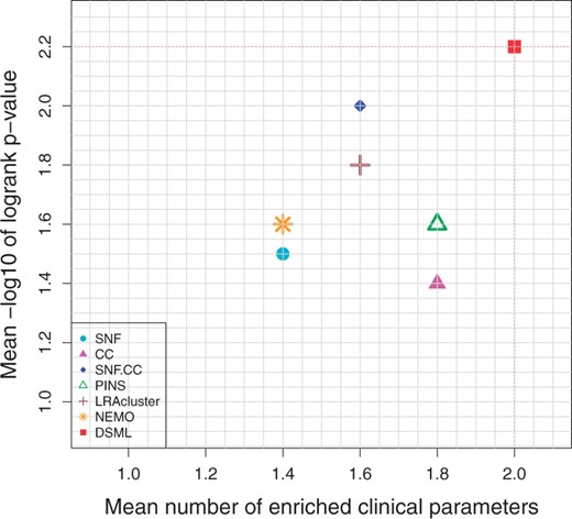
Mean performance of the different algorithms on five cancer datasets. Y-axis represents average −log10 logrank test’s P-values and X-axis represents average number of enriched clinical parameters in the clusters. The red dotted lines highlight DSML’s performance
Prediction performance comparison of integrative algorithms on multi-omics cancer datasets
| Alg./cancer | BIC | COAD | GBM | KRCCC | LSCC | Mean |
|---|---|---|---|---|---|---|
| SNF | 2/1.7 | 1/0.3 | 1/3.2 | 2/1.0 | 1/1.3 | 1.4/1.5 |
| CC | 2/2.2 | 1/0.1 | 1/1.6 | 4/2.3 | 1/0.8 | 1.8/1.4 |
| SNF.CC | 2/3.8 | 1/0.4 | 1/2.9 | 3/0.9 | 1/1.8 | 1.6/2.0 |
| PINS | 3/3.4 | 1/0.4 | 1/2.7 | 3/0.3 | 1/1.2 | 1.8/1.6 |
| LRAcluster | 3/2.0 | 1/0.3 | 1/1.6 | 2/3.8 | 1/1.1 | 1.6/1.8 |
| NEMO | 2/1.9 | 1/0.1 | 1/3.9 | 2/1.1 | 1/1.2 | 1.4/1.6 |
| DSML | 3/3.9 | 1/1.0 | 2/2.3 | 3/1.9 | 1/1.9 | 2.0/2.2 |
Note: Within each cell, the first number indicates significant clinical parameters detected, the second number is −log10 P-value for survival, 0.05 is selected as the threshold for significance and the significant results are shown in bold. Mean is algorithm average.
To evaluate the robustness of the proposed DSML to varying parameter , we select its value from the candidate set and execute DSML on the BIC cancer dataset with three-omics. Figure 4 shows the number of significantly enrichment and −log10 logrank P-value with varying . It can be seen from the figure that changing has a little effect on the prediction performance of cancers. Hence, we can conclude that DSML is relatively robust to the choice of .
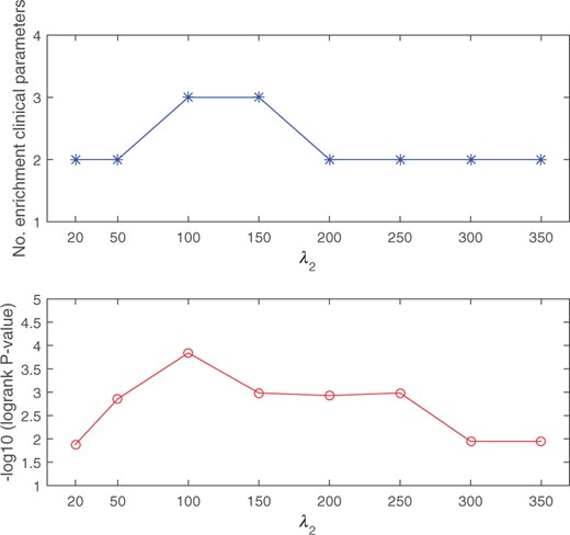
Robustness analysis for DSML
3.2 Partial-level omics datasets
In order to evaluate the performance and the flexibility of the algorithm on partial-level omics datasets, we apply DSML in two scenarios.
In the first scenario, only single-level omics data are available at diagnosis. Since branch parts in DSML communicate with and learn from each other in training stage, the weights in single branch networks have contained the information from multiple omics data. Thus, even though there is only one omics data at diagnosis stage, the branch part can still handle this situation. Specifically, the corresponding branch part within the trained DSML is adopted to obtain the similarity matrix among given single-level data. Then, spectral clustering based on this similarity matrix is utilized to identify cancer subtypes. We select conventional spectral clustering on original single-level data for comparisons. Comparison results are presented in Table 2. It is obvious that the performance of clustering using similarity matrix obtained by branch model is much better than it only obtained by original single-level data. This phenomenon indicates that the use of mutual learning mechanism can significantly improve the ability of data representation for subtype prediction. Even though only one level data is used for subtype’s prediction, it still archives satisfactory results by using DSML.
Prediction performance comparison of spectral clustering and branches within DSML on each single omics data
| Spectral clustering | Branches within DSML | |||||
|---|---|---|---|---|---|---|
| mRNA | miRNA | DNAm | mRNA | miRNA | DNAm | |
| BIC | 2/1.4 | 2/0.5 | 1/0.7 | 3/2.9 | 2/1.8 | 2/1.7 |
| COAD | 0/0.3 | 0/0.4 | 0/0.6 | 1/0.9 | 0/0.5 | 1/0.6 |
| GBM | 1/0.9 | 1/0.8 | 1/0.4 | 1/2.0 | 1/1.9 | 2/1.8 |
| KRCCC | 1/0.6 | 1/1.0 | 1/0.1 | 2/1.9 | 1/2.0 | 2/1.9 |
| LSCC | 1/0.2 | 1/0.5 | 1/0.3 | 1/1.0 | 1/0.9 | 1/1.7 |
| Mean | 1.0/0.7 | 1.0/0.6 | 0.8/0.4 | 1.6/1.7 | 1.0/1.4 | 1.6/1.5 |
Note: mRNA, miRNA and DNAm denote mRNA expression, miRNA expression and DNA methylation data, respectively. The numbers in each cell have the same meaning as in Table 1.
In the second scenario, some patients loss omics measurements. In experiments, we randomly sampled a fraction θ of the patients and removed their mRNA expression, as described in NEMO (Rappoport and Shamir, 2019). This procedure is repeated five times. The survival analysis and enrichment of clinical labels are still adopted to measure the quality of the prediction solutions. Average results of DSML and NEMO on all five cancer types are shown in Figure 5. The figure reveals that DSML gives a better performance than NEMO with respect to survival and enrichment analysis under all missing rates. These results suggest that DSML can be robustly applied to partial-level omics datasets.
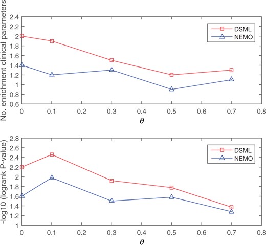
Average performance as a function of the fraction of samples missing data in mRNA expression. The top plot shows the results of enriched clinical parameters and the bottom plot shows the results of survival analysis
In general, the proposed DSML can obtain the cancer subtypes with statistically significant difference in survival profiles and significant clinical enrichment. Moreover, DSML can effectively solve the problem of partial-level omics data. Hence, DSML is a powerful framework for predicting cancer subtypes.
4 Conclusion
Cancer subtypes prediction plays an important role in personalized medicine framework, since stratifying patients correctly into subtypes can provide more targeted treatment and it would ultimately lead to better survival rates of patients. Integrating multiple level omics data can significantly improve clinical outcome predictions, since cancer is a phenotypic end-point incident cumulated via multiple levels in biological system from genome to proteome. In this study, a method called DSML has been proposed for subtype’s prediction by integrating multi-level omics data. DSML employs deep neural networks by incorporating subspace learning and mutual learning to recover the intrinsic similarity relationships among intra-level and across level data, and then adopts spectral clustering to predict patient subtypes. DSML can extract discriminative features simultaneously from multiple branch parts and fuze features via main-stem part. The mutual learning strategy provides an effective solution to the problem of partial-level data missing. Experimental results on five TCGA multiple omics datasets clearly indicate that DSML has better integrative performance compared to other relevant technologies. Moreover, DSML also effectively overcomes the prediction issues related to single-level omics data and partial-level omics data. Thus, DSML is a more general framework for multi-level omics data integrative analysis. As a scope of future work, we plan to involve protein–protein interaction networks to improve the interpretability of integrative strategy.
Acknowledgements
We would like to thank Shuhui Liu for useful conversations. We are grateful to anonymous reviewers for their many helpful and constructive comments that improved the presentation of the article.
Funding
This work was supported by National Natural Science Foundation of China (NSFC) Grant (61806159, 61972312); Xi’an Municipal Science and Technology Program (2020KJRC0027); Natural Science Basic Research Program of Shaanxi (2020JM-575); and Doctoral Scientific Research Foundation of Xi’an Polytechnic University (BS202108).
Conflict of Interest: none declared.

