


Abstract
Knowledge of protein-binding residues (PBRs) improves our understanding of protein−protein interactions, contributes to the prediction of protein functions and facilitates protein−protein docking calculations. While many sequence-based predictors of PBRs were published, they offer modest levels of predictive performance and most of them cross-predict residues that interact with other partners. One unexplored option to improve the predictive quality is to design consensus predictors that combine results produced by multiple methods.
We empirically investigate predictive performance of a representative set of nine predictors of PBRs. We report substantial differences in predictive quality when these methods are used to predict individual proteins, which contrast with the dataset-level benchmarks that are currently used to assess and compare these methods. Our analysis provides new insights for the cross-prediction concern, dissects complementarity between predictors and demonstrates that predictive performance of the top methods depends on unique characteristics of the input protein sequence. Using these insights, we developed PROBselect, first-of-its-kind consensus predictor of PBRs. Our design is based on the dynamic predictor selection at the protein level, where the selection relies on regression-based models that accurately estimate predictive performance of selected predictors directly from the sequence. Empirical assessment using a low-similarity test dataset shows that PROBselect provides significantly improved predictive quality when compared with the current predictors and conventional consensuses that combine residue-level predictions. Moreover, PROBselect informs the users about the expected predictive quality for the prediction generated from a given input protein.
PROBselect is available at http://bioinformatics.csu.edu.cn/PROBselect/home/index.
Supplementary data are available at Bioinformatics online.
1 Introduction
Protein−protein interactions (PPIs) drive many cellular functions including signaling, catalysis, metabolism and regulation of the cell cycle (Braun and Gingras, 2012; Figeys, 2002). Knowledge of PPIs contributes to the development of PPI networks (De Las Rivas and Fontanillo, 2012), which in turn empowers prediction of protein function (Ahmed et al., 2011; Hou, 2017; Orii and Ganapathiraju, 2012; Zhang et al., 2019). Analysis of PPI sites provides molecular-level insights into mechanisms of human diseases (Kuzmanov and Emili, 2013; Nibbe et al., 2011; Zinzalla and Thurston, 2009). These sites are nowadays targeted for the development of therapeutics (Johnson and Karanicolas, 2013; Petta et al., 2016; Sperandio, 2012). Elucidation of novel PPIs is supported by computational predictors (Aumentado-Armstrong et al., 2015; Esmaielbeiki et al., 2016; Maheshwari and Brylinski, 2015; Xue et al., 2015; Zhang and Kurgan, 2018). We concentrate on the methods that perform predictions directly from protein sequences, which are readily available for thousands of sequences genomes. The sequence-based methods are categorized into two groups depending on their output: protein-level predictors that predict whether proteins interact with each other versus residue-level methods that predict protein-binding residues (PBRs) (Zhang and Kurgan, 2018).
We focus on the sequence-based predictors of PBRs that arguably provide more detailed information than the other class of predictors. So far, 18 of these predictors were developed. They include (in chronological order): ISIS (Ofran and Rost, 2007), SPPIDER (Porollo and Meller, 2006), predictors by Du et al. (2009) and Chen and Jeong (2009), PSIVER (Murakami and Mizuguchi, 2010), predictor by Chen and Li (2010), HomPPI (Xue et al., 2011), LORIS (Dhole et al., 2014), SPRINGS (Singh et al., 2014), methods by Wang et al. (2014) and Geng et al. (2015), CRF-PPI (Wei et al., 2015), PPIS (Liu et al., 2016), iPPBS-Opt (Jia et al., 2016), SPRINT (Taherzadeh et al., 2016), SSWRF (Wei et al., 2016), SCRIBER (Zhang and Kurgan, 2019) and DeepPPISP (Zeng et al., 2020). These predictors find various practical applications in the context of functional characterization of proteins (Banadyga et al., 2017; Burgos et al., 2015; Mahboobi et al., 2015; Mahita and Sowdhamini, 2017; Wiech et al., 2015; Yang et al., 2017; Yoshimaru et al., 2017), estimation of binding affinities (Lu et al., 2018) and development of personalized medicine platforms (Hecht et al., 2015). They utilize a diverse assortment of predictive models that rely on a wide range of algorithms (sequence alignment, neural networks, support vector machines, random forest, etc.) and predictive inputs [sequence, evolutionary conservation (ECO), putative solvent accessibility, etc.] (Zhang and Kurgan, 2018). While recent studies reveal that this area has progressed over the last decade (Zhang and Kurgan, 2018, 2019), the predictive performance remains modest and majority of methods struggle with cross-prediction (Zhang and Kurgan, 2018). The latter means that they often predict residues that interact with other ligands (e.g. DNA and RNA) as PBRs. In spite of the availability of a large and diverse population of predictors and the modest predictive quality, the development of consensus-based approaches was not yet tackled in this area. The consensus methods use a collection of results produced by base predictors to produce new prediction that offers better predictive performance relative to the performance of the base methods. This approach was successfully deployed in several related areas (Kulshreshtha et al., 2016; Peng and Kurgan, 2012; Puton et al., 2012; Yan et al., 2016). For instance, there are numerous consensus methods for the sequence-based prediction of the intrinsically disordered residues (Meng et al., 2017a, b), and they are among the most accurate in this area (Fan and Kurgan, 2014; Monastyrskyy et al., 2014; Necci et al., 2017).
We address two objectives. First, we perform a comprehensive comparative analysis of predictive performance for a set of nine representative predictors of PBRs. In contrast to the prior studies where predictors were assessed using datasets-level results, we are the first to address evaluation at the arguably more practical protein-level, i.e. user typically apply these tools to predict individual proteins. Combination of dataset- and protein-level analyses allows us to formulate original and interesting observations concerning overall predictive performance, severity of cross-predictions, complementarity between predictors and factors that determine predictive quality. Second, we utilize these insights to develop an innovative consensus architecture that delivers improved predictive performance. Our design significantly improves over the base methods and estimates the expected predictive performance of the resulting protein-level prediction.
2 Materials and methods
2.1 Selection of a representative set of current predictors
Similar to the recent comparative review (Zhang and Kurgan, 2018), the criteria used to select representative predictors are: (i) availability (at minimum either webserver or source code is provided); (ii) scalability (prediction for an average size protein chain must complete inside 30 min); and (iii) outputs must include both binary predictions (each residue is categorized as PBR versus non-PBR) and numeric propensity for protein binding. The propensities provide more granular information that allows calibration of the amount of predicted PBRs and are required to estimate commonly used predictive performance measures. Nine methods satisfy these requirements: SPPIDER (Porollo and Meller, 2006), PSIVER (Murakami and Mizuguchi, 2010), LORIS (Dhole et al., 2014), SPRINGS (Singh et al., 2014), CRF-PPI (Wei et al., 2015), SPRINT (Taherzadeh et al., 2016), SSWRF (Wei et al., 2016), SCRIBER (Zhang and Kurgan, 2019) and DeepPPISP (Zeng et al., 2020). They are summarized in Supplementary Table S1. Importantly, this list includes all recently published tools.
2.2 Benchmark dataset
We use the dataset that was published in Zhang and Kurgan (2019) and which was collected using the procedure from Zhang and Kurgan (2018). In contrast to prior datasets in this area, this dataset annotates a broad range of protein−ligand interactions (allowing us to comprehensively evaluate cross-predictions) and provides a more complete annotation of native-binding residues. The latter is accomplished by combining annotations collected across multiple complexes that share the same protein (Zhang and Kurgan, 2018). The source data were collected from the BioLip database (Yang et al., 2012) that annotates PBRs based on high-resolution structures of protein−protein complexes from PDB. Importantly, proteins in this dataset share low, <25%, similarity with the proteins in the training datasets of the selected nine representative predictors. This was done by clustering the set of the BioLip-annotated proteins combined with the training proteins collected from the nine studies using Blastclust at 25% sequence similarity (Altschul et al., 1997), and selecting proteins from the clusters that do not include the training proteins. This provides for a fair comparison (no method has an advantage of using similar proteins in their training process) and ensures that evaluation focuses on the proteins that cannot be accurately predicted with sequence alignment to the training proteins. The dataset includes 448 proteins with 101 754 residues that include 336 proteins that have PBRs and 112 that do not have PBRs but which interact with other ligands (DNA, RNA and a range of small molecules); the latter is crucial to assess the cross-predictions. We divide these proteins at random into two equal-sized subsets, TRAINING and TEST datasets, for the purpose of designing and testing the consensus predictor. Supplementary Table S2 summarizes the contents of these datasets and quantifies the amount of protein-, RNA-, DNA- and small ligand-binding residues. The annotated datasets are available at http://bioinformatics.csu.edu.cn/PROBselect/home/index.
2.3 Evaluation setup
We evaluate the putative propensities with the area under receiver operating characteristic curve (AUC). The curve plots TPR (true positive rate) = TP/(TP + FN) against FPR (false positive rate) = FP/(FP + TN) that are computed by binarizing the propensities using thresholds equal to all unique values of the propensities.
2.4 Estimation of predictive quality from protein sequence
As part of the comparative evaluation, we show that predictive performance of the considered methods varies widely between proteins, and that different methods perform well for different protein sets. We also found that the predictive quality of specific methods can be linked to biophysical and structural characteristics of proteins that can be computed directly from the sequences. In other words, specific predictors perform particularly well (poorly) for proteins that have certain sequence-derived biophysical and structural features. Thus, we hypothesize that we can accurately model the relation between these features and the predictive performance measured with the AUC for a particular predictor. We designed and trained models for four predictors that have high predictive performance (LORIS, SPRINGS, CRFPPI and SSWRF). We were unable to generate accurate models for the remaining five methods since their predictive quality is relatively low and thus cannot be reliably predicted.
Prediction of the AUC values from the sequence is three-step process. First, the input protein sequences are used to generate sequence profile that describes relevant physiochemical and structural features of the constituent residues. Second, the profiles are converted into vectors of numeric features that aggregate and combine the physiochemical and structural information at the protein level. Third, the feature vectors are processed by the regression models that predict the AUC values. The following subsections detail these three steps.
2.4.1 Sequence profile
The physiochemical and structural features that were found in the literature to be relevant to protein−ligand interactions include (Zhang et al., 2019): residue-level propensity for binding (some amino acids are more prone to interact with specific partner types), solvent accessibility (PBRs are located on protein surface), ECO (PBRs tend to be conserved in the sequence), secondary structure, hydrophobicity, polarity (polar residues are more likely to interact with proteins and DNA) and charge (charged residues are more likely to interact with nucleic acids). We use these characteristics to develop the sequence profile. The relative amino acid propensities (RAAP) for interactions with proteins, DNA and RNA were collected from Zhang et al. (2019). The relative solvent accessibility (RSA) was predicted from sequence using the accurate and quick ASAquick method (Faraggi et al., 2014). The ECO values were generated from the sequence with the fast and sensitive HHblits (Remmert et al., 2012). The secondary structure was predicted from the sequence using the fast version of the popular PSI-PRED method which does not use the multiple sequence alignments (Buchan et al., 2013). We also predicted the disordered protein-binding residues with the with computationally efficient and popular ANCHOR tool (Dosztanyi et al., 2009). Finally, the physiochemical properties (hydrophobicity, polarity, polarizability and charge) were quantified using the AAindex database (Kawashima et al., 2007). The computation of the profile is fast as we rely on the computationally efficient algorithms.
2.4.2 Conversion of the profile into protein-level feature vector
The sequence and sequence profile, where each amino acid is described by the above-mentioned physiochemical and structural characteristics, are converted into a vector of protein-level numeric features. This conversion is necessary to train regression models. The vector includes the composition of the 20 amino acid types; sequence length; the average over the residues in the sequence for the putative RSA, ECO, polarity, polarizability, charge, hydrophobicity, putative propensity for disordered protein binding, and RAAP for interactions with proteins, DNA and RNA; fraction of putative surface residues, conserved residues, positively and negatively charged residues, putative disordered protein-binding residues, and putative coil, strand and helix residues. We also designed features that combine multiple characteristics including RAAP for protein/DNA/RNA interactions for the putative surface residues; physiochemical properties and ECO of the putative surface residues; RAAP for protein/DNA/RNA interactions for the conserved residues; and RAAP for protein/DNA/RNA interactions for the putative surface residues that are conserved. Supplementary Table S3 details calculation of the corresponding set of 65 features.
An alternative to this feature-based approach is to process the profile using a deep neutral network, as it was recently done to predict PBRs (Zeng et al., 2020). However, this approach has underperformed when compared with other methods that rely on the conversion of the input profile into feature vectors (Table 1; these results are discussed in Section 3.1).
Comparison of the predictive performance of nine representative predictors of PBRs on the benchmark dataset
| Predictor | AUC | Sensitivity | FPR (sensitivity to FPR rate) | FCPR (sensitivity to FCPR rate) | ||||
|---|---|---|---|---|---|---|---|---|
| Dataset-level | Median per-protein | Dataset-level | Median per-protein | Dataset-level | Median per-protein | Dataset-level | Median per-protein | |
| CRFPPI | 0.683 | 0.706 | 0.271 | 0.261* | 0.113 [2.4] | 0.097= [2.7] | 0.204 [1.3] | 0.182* [1.4] |
| SSWRF | 0.693 | 0.701= | 0.311 | 0.295* | 0.113 [2.8] | 0.105= [2.8] | 0.210 [1.5] | 0.191* [1.5] |
| LORIS | 0.657 | 0.671* | 0.266 | 0.260* | 0.114 [2.3] | 0.109= [2.4] | 0.192 [1.4] | 0.167* [1.6] |
| SPRINGS | 0.626 | 0.646* | 0.234 | 0.219* | 0.120 [2.0] | 0.103= [2.1] | 0.235 [1.0] | 0.212* [1.0] |
| SCRIBER | 0.717 | 0.635* | 0.311 | 0.192* | 0.093 [3.3] | 0.046 [4.2] | 0.100 [3.1] | 0.000 [inf] |
| SPRINT | 0.573 | 0.608* | 0.187 | 0.156* | 0.128 [1.5] | 0.110= [1.4] | 0.379 [0.5] | 0.409* [0.4] |
| PSIVER | 0.578 | 0.606* | 0.192 | 0.157* | 0.128 [1.5] | 0.108= [1.5] | 0.251 [0.8] | 0.200* [0.8] |
| DeepPPISP | 0.642 | 0.599* | 0.477 | 0.500 | 0.286 [1.7] | 0.360* [1.4] | 0.422 [1.1] | 0.500* [1.0] |
| SPPIDER | 0.513 | 0.486* | 0.198 | 0.125* | 0.132 [1.5] | 0.102= [1.2] | 0.323 [0.6] | 0.293* [0.4] |
Note: The methods are sorted by their median per-protein AUC values in the descending order. Methods indicated in bold font provide the best value of a given measure of predictive performance. We report medians of the per-protein values and assess significance of the differences between the per-protein values of the best method and each of the other methods.
Statistically significant differences (P-value <0.001), while ‘=’ denotes differences that are not significant (P-value ≥ 0.001). We use paired t-test (for normal data) or Wilcoxon test (otherwise) and we assess normality with the Kolmogorov−Smirnov test.
2.4.3 Prediction by regression models
The features are used as an input to a regression model that predicts the predictive performance (quantified with AUC) for a given predictor of PBRs. We derive and optimize these models using two popular algorithms, linear regression (LR) and support vector regression (SVR). The optimization was done exclusively on the TRAINING dataset using 3-fold cross-validation with the aim to maximize quality of the AUC predictions. The predictive quality was quantified with three popular measures: Pearson’s correlation coefficient (PCC), mean absolute error (MAE) and root mean squared error (RMSE) between the predicted and the actual AUC values.
The optimization includes feature selection and parametrization of the regression algorithms. The feature selection aims to remove features that lack predictive power and to reduce redundancy, i.e. remove mutually correlated features. This is crucial for the LR algorithm that is sensitive to collinearity between the input features. We empirically compare two feature selection methods: model-specific approach and a wrapper-based selection. The first method relies on the popular lasso method that embeds feature selection into optimization of the LR model (Tibshirani, 1996). We parametrize the number of regularization coefficients in the lasso method by considering alpha = {1, 0.9, …, 0.1, 0.05, 0.01, 0.005, 0.001, 0.0005, 0.0001, 0.00005, 0.00001, 0.000005, 0.000001}. The second method is the wrapper-based feature selection (Kohavi and John, 1997) that was recently used in several related studies (Hu et al., 2019; Meng and Kurgan, 2018; Yan and Kurgan, 2017; Zhang and Kurgan, 2019). This approach selects feature sets that secure highest predictive quality when used with the corresponding predictive model. First, we rank features by their predictive performance when they are used to implement univariate LR or SVR models. Second, starting with the top-ranked (the most predictive) feature we incrementally add to the next-ranked feature to the set of selected features if this generates improvements in the predictive performance, i.e. the expanded feature set secures better performance than the set before this his feature was added; otherwise the next-ranked feature is skipped. We scan the sorted feature set once and we consider two ways to quantify predictive performance, using PCC and MAE values. Moreover, we perform grid search to parametrize the SVR model; we use the popular RBF kernel and we consider γ = {0.1, 0.2, …, 1}, and coefficient C = 2i where i = {−5, −4, …, 0, 1, …, 5}. In total, we consider four scenarios for LR (lasso and wrapper selection optimized to maximize PCC and to minimize MAE), four scenarios for SVR (wrapper selection and use of the complete feature set when maximizing PCC and minimizing MAE), and we separately optimize these models for each of the considered four predictors of PBRs: LORIS, SPRINGS, CRFPPI and SSWRF, as well as the consensus predictor PROBselect. The results are summarized in Supplementary Table S4. We conclude that the best results, as judged on the TRAINING dataset, are obtained with the SVR model that applies the complete feature set and which is parametrized to maximize PCC. This model secures the highest PCC for each of the five predictors combined with low MAE and RMSE values. The average (over the five predictors) PCC and MAE of this model are 0.44 and 0.083, respectively, compared with the second best option (SVR optimized to minimize MAE) that secures lower average PCC = 0.41 and slightly better average MAE = 0.081, and the best LR-based configuration that offers PCC = 0.39 and MAE = 0.084. Consequently, we apply the best-performing SVR models to implement the consensus predictor.
2.5 Design of the consensus predictor of PBRs
A traditional consensus design in related areas relies on combining the residue-level predictions generated by multiple predictors (Fan and Kurgan, 2014; Kulshreshtha et al., 2016; Peng and Kurgan, 2012; Puton et al., 2012; Yan et al., 2016). In other words, the predictions generated by multiple methods are combined together for each amino acid in the input protein sequence. We propose an innovative solution that draws from the dynamic classifier selection model (Cruz et al., 2018). In this model, one of the base predictors is selected on the fly for each new sample that is predicted. This works well if the selected predictor provides better results for this sample compared with the other input predictors. The dynamic classifier selection model was recently shown to improve over several other alternatives, including voting and boosting (Britto et al., 2014; Cruz et al., 2015; Woloszynski and Kurzynski, 2011).
We perform the ‘dynamic’ selection of the predictor that provides favorable predictive performance for at the protein level (i.e. our sample is the whole protein). The selection is implemented using the AUC values predicted by the SVR models, i.e. we select the predictor that secures the highest predicted AUC for a given protein sequence. This design takes advantage of two observations that we derived based on the protein-level assessment of the nine predictors of PBRs. First, two predictors, SSWRF and CRFPPI, secure the best and statistically significantly better levels of protein-level predictive performance when compared with the other seven predictors. Second, SCRIBER is the only method that accurately identifies proteins that do not have PBRs. More specifically, SCRIBER does not cross-predict PBRs and its FCPR value is statistically significantly better than FCPRs of the other eight predictors. Correspondingly, our consensus design, named PROBselect, uses three steps to make prediction for a given protein sequence (Fig. 1):
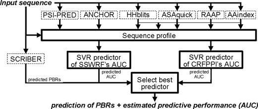
Flowchart of the PROBselect consensus predictor. Input and outputs are denoted with italic font. Elements with solid boundaries were developed in this article
Use SVR models to predict AUC of SSWRF and CRFPPI.
Generate predictions of PBRs using the SCRIBER method.
Select the predictor for the input protein as follows: use the prediction by SCRIBER if SCRIBER does not predict PBRs; otherwise use one of the other two methods that has higher predicted AUC value.
The determination whether SCRIBER predicts PBRs relies on its published false positive rate of 0.015 for the proteins that do not interact with other proteins (Zhang and Kurgan, 2019). In other words, if the fraction of the PBRs predicted by SCRIBER <0.015 then we assume that the input proteins does not bind other proteins (the PBR predictions are spurious). A unique benefit of our design, in contrast to the traditional residue-level consensus, is that we provide the estimate of the expected level of predictive performance (the SVR-predicted AUC value) besides providing the (dynamically selected) consensus prediction. This additional output informs the end users about reliability of the associated prediction. Importantly, our empirical tests (Section 3) reveal that this novel type of consensus produces higher predictive performance than its base predictors and traditional consensuses, and that the estimates of the AUC values that are produced by SVR models are relatively accurate and can be used to identify well-predicted proteins.
3 Results
3.1 Comparative analysis of predictive performance
We assess predictive performance of the nine representative predictors of PBRs on the benchmark dataset with 448 proteins. The dataset shares low sequence similarity with the training data used to develop these tools and includes a mixture of proteins that have PBRs and proteins that do not have PBRs but which interact with other ligands (nucleic acids and small molecules). This allows for a fair assessment that considers two important aspects of predictive performance: ability to correctly predict PBRs and ability to differentiate PPIs from interactions with the other ligands.
The results of the dataset-level evaluation of the nine predictors (Table 1) are consistent with the previous reports (Zhang and Kurgan, 2018, 2019). First, the most accurate predictors (AUC > 0.69) include SCRIBER, SSWRF and CRFPPI. Second, we note high FPR and FCPR (false positive rate among residues that interact with other ligands including nucleic acids and small molecules) values relative to the sensitivity/TPR values. Table 1 includes the sensitivity to FPR and sensitivity to FCPR rates inside the square brackets. Values of the rates ≤1 mean that a given tool makes relatively more false predictions than correct predictions. This is particularly troubling for the rate with FCPR since it means that comparable or larger rates of PBRs are predicted for the residues that bind other ligands when compared with the residues that bind proteins. In other words, predictors that have such rates indiscriminately predict all types of binding residues, not just PBRs. Only SCRIBER secures high FCPR rate equal 3.1. Three methods obtain rates between 1.3 and 1.5 (CRFPPI, SSWRF and LORIS) while the remaining tools have rates at or below 1.1. These results are in agreement with the findings in Zhang and Kurgan (2018), showing that majority of the current methods substantially cross-predict other types of interactions for PPIs. The main reason is that they have used training datasets that include only protein-binding proteins, without consideration for inclusion of residues that interact with other types of partners (Zhang and Kurgan, 2018).
3.2 Comparative analysis of protein-level predictions
We are the first to couple the traditionally done dataset-level assessment with first-of-its-kind evaluation for individual proteins, which is arguably the most common mode of use for these predictors. We are motivated by a recent study that investigated quality of protein-level predictions of intrinsic disorder, which produced several practical and novel observations (Katuwawala et al., 2020a). The raw distributions of the protein-level predictive performance are shown in Supplementary Figure S1, with the corresponding violin plots in Supplementary Figure S2. We report the median per-protein values in Table 1 and we provide the key distributions in Figure 2. For each measure, we evaluate significance of the differences in the protein-level performance between the best-performing method and the other eight predictors.
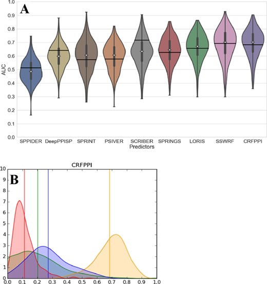
Distributions of the per-protein predictive performance measured for the nine representative predictors of PBRs on the benchmark dataset. Violin plots in (A) show distributions of the per-protein AUC values where the thick vertical lines represent the first quartile, median (white dot) and third quartile, whiskers denote the minimal and maximal values, and the black horizontal lines denote the dataset-level AUC. (B) The distributions of the AUC (in yellow), sensitivity (blue), FPR (red) and FCPR (green) values for the CRFPPI predictor that has highest median per-protein AUC; the vertical lines denote dataset-level values. The y-axis is the fraction of proteins for a given AUC, FPR, FCPR or sensitivity value
First, we observe that the overall performance quantified with AUC varies widely across proteins for each of the nine predictors (Fig. 2). For instance, while the dataset-level AUC of CRFPPI is 0.68, its per-protein AUC values range between 0.36 and 0.92, with a long tail for the low values and the peak at around 0.75. This means that while the users expect to receive predictions with AUC below 0.7 (based on this and prior benchmarks), in fact they often will be surprised with better results, but may also encounter very poor predictions for some proteins (AUC < 0.5, which is below random levels). Similarly, the protein-level sensitivity, FPR and FCPR values vary widely between proteins (Fig. 2B for CRFPPI; Supplementary Fig. S2B−D for the other predictors). The most worrying observation comes from comparing sensitivity and FCPR distributions. For several methods, including SPPIDER, PSIVER and SPRINT, the majority of proteins have FCPR values larger than sensitivity. That means that for these proteins they generate a larger fraction of PBRs among residues that bind other ligands when compared with the residues that in fact interact with proteins. We see that in Table 1 where the median protein-level sensitivity to FCPR rate for these methods is much below 1, i.e. 0.4 for SPRINT and SPPIDER and 0.8 for PSIVER.
The overall best protein-level predictor is CRFPPI, with median AUC = 0.706. The AUC values of the second best SSWRF are not significantly different (P-value = 0.08, median AUC = 0.701), while the improvements over the remaining seven predictors are statistically significant (P-value <0.001). The newest tool, DeepPPISP, secures the highest sensitivity but at the expense of similarly high FPR and FCPR, leading to a substantial over-prediction of PBRs. The more informative protein-level sensitivity to FPR rate and sensitivity to FCPR rate reveal a large advantage for SCRIBER. This method secures the lowest FPR and FCPR values, and by far the highest sensitivity to FPR and FCPR rates. The SCRIBER’s FPR and FCPR values are similar for both assessments, the protein- and dataset-level, which is in contrast to all other predictors for which FCPRs are much larger than FPRs. The latter demonstrates that the other eight methods over-predict PBRs among residues that interact with other ligands. This even includes the two overall-best methods, CRFPPI and SSWRF, for which the sensitivity to FCPR rates equal 1.4 and 1.5, respectively. We observe that directly in Figure 2B where the distribution of sensitivity values (blue line) is very close to the distribution of FCPR values (green line) for CRFPPI; the distribution for SSWRF is in Supplementary Figure S1. This suggests that while CRFPPI and SSWRF accurately predict PBRs for proteins that interact with protein partners (high AUC), they substantially cross-predict PBRs for the proteins that bind other ligand types (low rate to FCPR).
We further explore this important and often overlooked aspect in Supplementary Figure S3. This figure directly compares the rate of predicted PBRs between the 336 protein-binding proteins and the 112 proteins that bind other ligands (nucleic acids and small molecules) from our benchmark dataset. The two rates are virtually identical for several predictors, including SPPIDER, PSIVER, SPRINT, SPRINGS, LORIS and CRFPPI. This reveals that they are unable to differentiate between these two distinct protein sets. We note a marginal increase in the rate of prediction of PBRs for the protein-binding proteins for DeepPPISP and SSWRF. The only predictor for which the rate of PBRs is substantially higher for protein-binding proteins is SCRIBER. Overall, our analysis suggests that SCRIBER is the only method that escapes the cross-prediction curse and can be used to separate protein-binding proteins from proteins that interact with other partner types. This is consistent with the premise of this tool that was designed to reduce the cross-predictions (Zhang and Kurgan, 2019).
3.3 Complementarity of predictors of PBRs
The feasibility of the development of successful consensus predictors is dependent on complementarity of the base/input methods (Peng and Kurgan, 2012). Supplementary Figure S4 provides side-by-side comparison of the per-protein AUC values for the top five protein-level predictors from Table 1. The predictive performance for individual proteins ranges broadly across different predictors. The figure shows that the AUCs of the best-overall CRFPPI predictor are outperformed for many proteins by one of more other methods. Correspondingly, we measure the complementarity in two ways: (i) we investigate the ability of multiple methods to contribute high-quality predictions and (ii) we quantify the size of the protein set for which the consensus would not be able to provide good predictions.
First, we analyze whether the best predictions are primarily attributed to a single method or whether they are generated by multiple methods, each performing favorably for a relatively large protein set (Fig. 3A). The consensus would benefit from the latter scenario since appropriate selection of the best predictions across multiple tools would lead to a solution that improves over the predictions generated by the single best-overall tool. The outer ring in Figure 3A reveals that the largest set of proteins for which the same method (SSWRF) provides the best results (highest AUC) constitutes only 29% of the dataset. Interestingly, the optimal predictions for 73% of the proteins are generated by just three predictors: SSWRF, CRFPPI and SCRIBER. The remaining six methods cover only 27% of the proteins, with SPRING and SPPIDER producing the best results for only 2 and 1% of the proteins, respectively. The middle and inner rings in Figure 3A focus on the over-prediction (FPR) and cross-prediction (FCPR) aspects. SCRIBER has a clear advantage, as it produces predictions with the lowest FPR for 43% of proteins and the lowest FCPR for 37% of proteins. Several other methods are relatively evenly distributed but they cover no more that 20% each, with the second best coverage at 18% for the best FPR at 15% for the best FCPR for PSIVER.
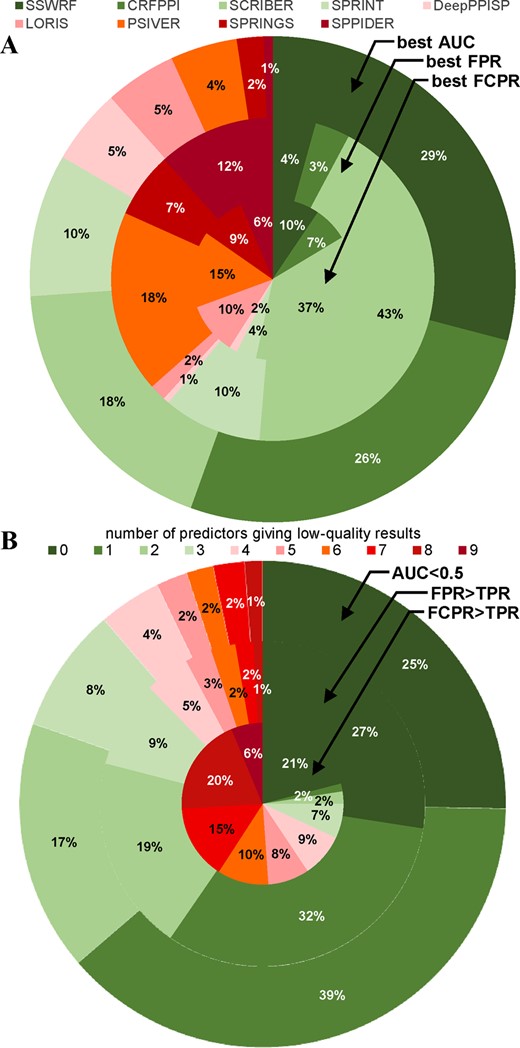
The best and the worst protein-level predictions across the nine predictors. (A) The fraction of proteins for which a given color-coded predictor secures the best predictive quality quantified with AUC (outer ring) FPR (middle ring) and FCPR (inner ring). (B) The fraction of proteins for which a given color-coded number of methods provides excessively low predictive performance. Outer ring defines low performance as AUC<0.5 (worse-than-random predictions). The middle ring defines low performance as significant over-prediction: FPR > TPR (proteins with the rate of correct PBR predictions below the rate of false positive predictions). The inner ring defines bad predictions as significant cross-prediction: FCPR > TPR (proteins with the rate of correct PBR predictions that is smaller than the rate of false positives among residues that interact with the other ligands)
Second, we analyze frequency of low-quality predictions across the nine methods. We aim to estimate the size of a protein set that cannot be accurately predicted with the current tools, and which therefore could be solved by the consensus. Figure 3B shows fraction of proteins for which a given color-coded number of methods provides low predictive performance. The outer ring focuses on proteins for which AUC is below random levels (<0.5). About 25% of proteins are predicted above random levels by all nine methods (dark green) and 79% are predicted better-than-random by majority of the methods (sum of all green fields). Moreover, each protein is predicted at the better-than-random level by at least one predictor, i.e. the dark red field is at 0% and is absent in the outer ring. The middle and inner rings focus on the proteins that are significantly over-predicted (FPR > TPR: proteins with the rate of correct PBR predictions below the rate of false positives) and significantly over-cross-predicted (FCPR > TPR: proteins with the rate of correct PBR predictions below the rate of false positives among residues that interact with other ligands), respectively. Figure 3B reveals that majority of the predictors does not significantly over-predict for 87% of proteins (all green fields in the middle ring in Fig. 3B), and at least one predictor does not significantly over-predict for each protein in the dataset (dark red field is absent). The inner ring reveals the significant impact of the wide-spread cross-predictions, i.e. only 21% of proteins are never significantly over-cross-predicted and majority of methods substantially over-cross-predicts 68% of proteins (sum of all non-green fields). The one method that provides relief in this aspect is SCRIBER. Availability of this tool is the reason why only 6% of proteins (dark red field) have this problem across all nine predictors.
To sum up, multiple methods contribute the best protein-level results and nearly all proteins can be predicted at better-than-random levels. This suggests that an effective consensus could be designed using current tools.
3.4 Estimation of predictive quality from protein sequence
Table 1 reveals that several current methods, such as SPPIDER, DeepPPISP, PSIVER and SPRINT, produce low quality results, i.e. low AUC and high FCPR. Figure 2A reveals that the predictive performance of the remaining methods varies widely across proteins, whereas Figure 3A further shows that they produce favorable results for distinct protein sets. We hypothesize that differences in the predictive performance of these well-performing methods is linked to intrinsic characteristics of the input protein chains. Supplementary Figure S5 shows relation between three example characteristics extracted from the sequence (average hydrophobicity, fraction of negatively charged residues and average propensity for protein-binding) and the AUC of the best-performing CRFPPI method. The hydrophobicity and propensity for protein binding are positively correlated with AUC of this predictor (PCC = 0.32 and 0.21, respectively) while the amount of negatively charged amino acids is negatively correlated (PCC = −0.33). These results suggest presence of a relation between the input protein chain and the predictive performance. Such relation could be used to estimate predictive performance of a given method directly from the sequence. Our hypothesis is also supported by a recent study that models these relations in the context of intrinsic disorder predictions (Katuwawala et al., 2020b).
We use 65 biophysical and structural features relevant to PPIs that are computed directly from the sequence. We model relation between these features and the AUCs using regression. We parametrized and selected a well-performing model that relies on support vector regression (SVR) using cross-validation on the TRAINING dataset; see Section 2 for details. Here, we assess performance of this model on the independent (low similarity) TEST set for the four well-performing predictors: SSWRF, CRFPPI, LORIS and SPRINGS (Table 2). We compare the SVR models to a current alternative that uses sequence alignment with the popular BLAST (Altschul et al., 1997; Hu and Kurgan, 2019), i.e. the AUCs of the most similar training proteins found with alignment are used as the prediction. We also compare against a random predictor that shuffles the actual AUC values obtained for the test proteins by a given predictor of PBRs—this way it predicts the correct distribution of the AUC values.
Comparison of predictive quality for the prediction of AUC values of the four accurate predictors of PBRs and PROBselect (Section 3.5) on the TEST dataset
| Predictor | SSWRF | LORIS | CRFPPI | SPRINGS | PROBselect | Average | |
|---|---|---|---|---|---|---|---|
| SVR models | PCC | 0.44 | 0.42 | 0.41 | 0.35 | 0.44 | 0.41 |
| MAE | 0.09 | 0.08 | 0.09 | 0.09 | 0.09 | 0.09 | |
| RMSE | 0.12 | 0.11 | 0.11 | 0.11 | 0.11 | 0.11 | |
| Alignment with BLAST | PCC | 0.09 | 0.06 | 0.04 | 0.03 | 0.06 | 0.06 |
| MAE | 0.12 | 0.11 | 0.11 | 0.11 | 0.11 | 0.11 | |
| RMSE | 0.15 | 0.14 | 0.15 | 0.14 | 0.14 | 0.15 | |
| Random predictor | PCC | −0.02 | 0.05 | −0.03 | 0.02 | 0.01 | 0.01 |
| MAE | 0.13 | 0.12 | 0.12 | 0.12 | 0.12 | 0.12 | |
| RMSE | 0.17 | 0.15 | 0.16 | 0.15 | 0.16 | 0.16 |
Notes: The support vector regression (SVR) model optimized using cross-validation on the TRAINING set is compared against an alignment approach and a baseline random predictor. We report Pearson’s correlation coefficient (PCC), mean absolute error (MAE) and root mean squared error (RMSE). The results in bold font are the best for a given measure. The last column is average over the five methods.
Table 2 shows that the SVR models produce accurate estimates of the predictive performance for the four predictors of PBRs, which are consistent with the cross-validation results on the TRAINING dataset (Supplementary Table S4). The average (over the four models) PCC = 0.41 and the average MAE = 0.09. These results are significantly better than the predictive performance offered by the two alternatives (P-value <0.01), where the average (over the four models) PCC <0.06 and the average MAE ≥ 0.11.
Next, we use the results produced by the SVR models in a practical context to identify well-predicted proteins. First, based on the results from Table 1 and Figure 3A, which suggests that the four methods for which we produced SVR models significantly cross-predict PBRs, we use SCRIBER to identify proteins that do not interact with proteins. These proteins are poorly predicted (due to cross-prediction) by these four tools. We use a simple filter to identify these problematic proteins, i.e. a given protein is assumed not to bind proteins if SCRIBER’s prediction includes a negligible amount of putative PBRs, i.e. the fraction of predicted PBRs <0.015, which corresponds to the expected SCRIBER’s FPR that was published in Zhang and Kurgan (2019). We replace the prediction generated by a given predictor (SSWRF, CRFPPI, LORIS and SPRINGS) with the SCRIBER’s prediction for these proteins. The effect of this filter can be quantified by comparing the ‘entire dataset with no SCRIBER’ and ‘entire dataset no SCRIBER’ points in Figure 4. The dataset-level AUC for CRFPPI increases from 0.69 to 0.72, for CRFPPI from 0.69 to 0.72, for LORIS from 0.65 to 0.67, and for SPRINGS from 0.62 to 0.65. Second, we sort proteins based on their corresponding SVR-predicted AUC values and we compare their actual dataset-level AUCs (Fig. 4). The points on the left side of Figure 4 corresponds to the subsets of the test proteins with progressively higher values of predicted AUC. We note a consistent trend (across the four methods) where proteins with higher putative AUCs are in fact predicted better. The left-most point reveals that the 10% of proteins in the TEST set identified by the SVR models as the most accurately predicted have in fact substantially higher AUC when compared with the overall AUC on the complete dataset. For CRFPPI, these proteins are predicted by with AUC = 0.74 compared with the overall AUC = 0.69. We observe similar differences for the other three predictors: 0.71 (top 10%) compared with 0.62 (complete dataset) for SPRINGS, 0.70 − 0.65 for LORIS, and 0.75 − 0.69 for SSWRF. Overall, we show that the four SVR models can be used to accurately identify well-predicted proteins.
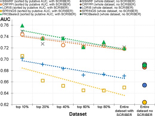
The dataset-level AUCs for subsets of the test proteins sorted based on their putative AUCs generated by the SVR models. We consider subsets of test proteins for which the predicted AUCs are above a given percentile of all estimated AUCs, i.e. ‘top 10%’ corresponds the test proteins that have AUCs above the 90th percentile of the predicted AUCs. The two right-most points are the result on the complete TEST set where the ‘Entire dataset’ denotes the results of a given predictor on the complete test set with the use of the SCRIBER-based filter; ‘no SCRIBER’ are the results without the filter. Dotted lines are linear fit into the measured data
3.5 Consensus prediction of PBRs
We show that only a few methods secure high AUC values and that they predict well for different protein sets (Table 1; Fig. 3A). We found that SCRIBER effectively identifies proteins that do not have PBRs for which the other predictors suffer heavy cross-predictions (Table 1; Fig. 4). Finally, we developed SVR models that use protein sequence to accurately estimate predictive performance of the well-performing methods. These findings motivate the design of our consensus approach that applies the dynamic classifier selection approach (Cruz et al., 2018). Our PROBselect consensus (Fig. 1) works in three steps: (i) apply SVR models to predict AUCs of the two most accurate (and statistically not different) predictors: SSWRF and CRFPPI; (ii) generate predictions of PBRs with SCRIBER and (iii) dynamically select the optimal predictor as follows: use SCRIBER’s prediction if it identifies that the input protein does not have PBRs; otherwise use the predictor (SSWRF or CRFPPI) that secures higher SVR-predicted AUC. A unique advantage of our solution is the provision of the estimated AUC value that can be used to gauge the quality of the associated prediction.
We compare the PROBselect’s predictive performance against its base methods (SSWRF and CRFPPI, which significantly outperform the other seven methods; Table 1) and two implementations of traditional consensuses on the TEST dataset (Fig. 5). The traditional consensuses, which are popular in related protein bioinformatics areas, combine residue-level predictions generated by multiple predictors (Fan and Kurgan, 2014; Puton et al., 2012; Yan et al., 2016). We implemented the traditional consensus that combines two base method (SSWRF and CRFPPI) and the consensus that combines the nine predictors of PBRs. PROBselect secures the highest AUC = 0.720 ± 0.006 (Fig. 5), and outperforms the second best classical consensus with nine predictors (AUC = 0.704 ± 0.004; P-value <0.001) and the best base predictor, SSWRF (AUC = 0.691 ± 0.007; P-value <0.001). The ROC curves are shown in Supplementary Figure S6. The improvements offered by PROBselect in the sensitivity to FCPR rate, which quantifies ability to handle cross-predictions (we further explain this rate in Section 3.1), are also statistically significant (P-value <0.001). PROBselect secures rate = 1.98 ± 0.02 compared with the second best CRFPPI with rate = 1.46 ± 0.04. The traditional consensus with nine predictors, which obtains the second highest AUC, has much lower rate of 1.31 ± 0.02.
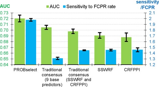
Comparison of predictive performance of the PROBselect consensus with two traditional consensuses that apply the two best (SSWRF and CRFPPI) and the nine predictors of PBRs, and the performance of SSWRF and CRFPPI—the two base methods used in PROBselect. We bootstrap the predictions (10 repetitions of 80% of proteins from the TEST dataset) and we assess significance of the differences in the AUC and sensitivity to FPCR rate values between the PROBselect and the other four methods using paired t-test; the measured data are normal based on the Kolmogorov−Smirnov test. The bars represent averages of the 10 results; whiskers show the standard deviations
In the spirit of the protein-level assessment theme of our article, we further assess PROBselect based on protein-level ranking of the quality of the predictions that it produces, relative to the quality of the predictions produced the nine currently available predictors (Table 3). We also include the oracle method that always select the most accurate results among all predictors. We rank quality of results produced by these 11 approaches for each protein, from best to worst, and we compare the average and median ranks across the proteins in the TEST set. The oracle is by default always the best and thus it secures rank of 1. The PROBselect obtains the second best rank at 3.4 (average) and 3 (median), which is substantially better than the third-best CRFPPI with 4.1 (average) and 4 (median) rank. This means that PROBselect’s predictions are expected to outperform results generated by the other predictors when applied at the protein level.
Average and median per-protein rank of the quality of predictions produced by the nine predictors of PBRs, the PROBselect consensus and the oracle predictor that always select the best prediction among the available nine predictors on the TEST dataset
| Methods | Oracle | PROBselect | CRFPPI | SSWRF | SCRIBER | LORIS | SPRINGS | PSIVER | SPRINT | DeepPPISP | SPPIDER |
|---|---|---|---|---|---|---|---|---|---|---|---|
| Average rank | 1.0 | 3.4 | 4.1 | 4.3 | 5.4 | 5.4 | 6.5 | 7.2 | 7.6 | 8.1 | 9.1 |
| Median rank | 1 | 3 | 4 | 4 | 6 | 5 | 7 | 8 | 8 | 9 | 10 |
Note: Lower rank is better.
We develop the SVR-based model that predicts AUC of the PROBselect from the input protein chain (details in Section 3.4). Table 2 shows that this models accurately estimates the predictive performance of PROBselect, with PCC = 0.44 and MAE = 0.09. These values are comparable to the results on the training dataset (Supplementary Table S4) and to the SVR models for SSWRF and LORIS, and are significantly better than the alignment and random predictor (P-value <0.01). Moreover, Figure 4 shows that the use of SCRIBER as a filter for PROBselect results in a substantial increase in AUC. The dataset-level AUC increases from 0.69 (‘no SCRIBER’) to 0.72 (‘with SCRIBER’). This figure also reveals that proteins with higher SVR-predicted AUCs are in fact predicted better by PROBselect. The left-most point shows that the 10% of the test proteins that the SVR models predicts as the most accurate secure AUC = 0.76. Furthermore, the linear trend for the PROBselect’s SVR model is better/above than the corresponding trends for the current predictors.
3.6 PROBselect webserver
A webserver the implements PROBselect is freely available at http://bioinformatics.csu.edu.cn/PROBselect/home/index. It allows for batch prediction of up to 5 FASTA-formatted protein chains. It requires about 1 min to predict an average-length sequence. Upon completion of the predictions, it sends link to the results to the user-provided email address. The output includes the prediction from SCRIBER, the estimated AUCs for SSWRF and CRFPPI, and the link to the webserver of the recommended predictor, i.e. the predictor that secures the highest predicted AUC. The results are available via a private HTML page (the URL is sent by the email) and via a parsable comma-separated text file with results.
4 Summary and conclusions
We perform first-of-its-kind comparative evaluation of the predictive performance of nine representative predictors of PBRs that focuses on the protein-level results. We find that the overall performance quantified with AUC varies widely across proteins, ranging from near-random or sub-random levels to very strong predictions, with AUC > 0.9 achieved by SSWRF and CRFPPI methods (Fig. 2A). The overall two best-performing predictors, CRFPPI and SSWRF, secure the median per-protein AUC of 0.70. While their predictive quality is statistically equivalent, they outperform the other current methods by a statistically significant margin.
We confirm conclusions from the recent reports (Zhang and Kurgan, 2018, 2019), which show that virtually all current predictors suffer substantial amounts of cross-predictions. This means that they often mis-predict residues that interact with nucleic acids and small molecules as PBRs. We show that for some methods, including SPPIDER, PSIVER and SPRINT, their rate of protein-level cross-predictions is higher than the rate of correct PBR predictions. Even the two best-overall predictors (CRFPPI and SSWRF) cross-predict at the 1:1.4 (for CRFPPI) and 1:1.5 (for SSWRF) rate, i.e. one cross-predicted residue for 1 correctly predicted PBR. The only method that successfully avoids the cross-prediction curse is SCRIBER, which secures median protein-level AUC = 0.64 while reducing the median amount of cross-predictions to zero. This suggests that SCRIBER can be used to accurately identify proteins that do not interact with proteins but which may interact with other partner types.
Our empirical analysis reveals that the predictive performance of the few well-performing predictors (CRFPPI, SSWRF, SPRINGS and LORIS) varies widely across proteins while producing favorable results for distinct protein sets. This suggests that the performance can be (at least partially) determined from the protein sequence. We designed and empirically tested SVR-based models that accurately estimate AUC of the above four methods and PROBselect from the sequence. Subsequently, we designed and empirically tested a novel consensus predictor of PBRs, PROBselect, which relies on these SVR models and the ability of SCRIBER to identify the proteins that do not interact with proteins. We demonstrate that our novel consensus design, which relies on the dynamic classifier selection approach, outperforms its base predictors and traditionally designed consensuses by a statistically significant margin. An important and unique advantage of PROBselect is the availability of the estimated AUC value that accompanies the prediction of PBRs and which informs the users about the expected predictive quality of this prediction.
Funding
This work was supported in part by the National Natural Science Foundation of China (grant 61832019) and the 111 Project (grant B18059).
Conflict of Interest: none declared.
Data availability
The data underlying this article are available in the article and in its online supplementary material.
References
Singh,

