


Abstract
Despite the fact that structural variants (SVs) play an important role in cancer, methods to predict their effect, especially for SVs in non-coding regions, are lacking, leaving them often overlooked in the clinic. Non-coding SVs may disrupt the boundaries of Topologically Associated Domains (TADs), thereby affecting interactions between genes and regulatory elements such as enhancers. However, it is not known when such alterations are pathogenic. Although machine learning techniques are a promising solution to answer this question, representing the large number of interactions that an SV can disrupt in a single feature matrix is not trivial.
We introduce svMIL: a method to predict pathogenic TAD boundary-disrupting SV effects based on multiple instance learning, which circumvents the need for a traditional feature matrix by grouping SVs into bags that can contain any number of disruptions. We demonstrate that svMIL can predict SV pathogenicity, measured through same-sample gene expression aberration, for various cancer types. In addition, our approach reveals that somatic pathogenic SVs alter different regulatory interactions than somatic non-pathogenic SVs and germline SVs.
All code for svMIL is publicly available on GitHub: https://github.com/UMCUGenetics/svMIL.
Supplementary data are available at Bioinformatics online.
1 Introduction
Pan-cancer genome sequencing projects, such the TCGA and PCAWG, have yielded unprecedented insights into the catalogue of somatic mutations in cancer genomes. Results from these efforts revealed that, on average, cancer genomes contain between four and five driver mutations (Campbell et al., 2020). The majority of these drivers are within the coding region of the genome. However, due to whole genome sequencing it is now clear that non-coding drivers also play an important role in cancer initiation and progression, although such driving non-coding events are scarcer than may be anticipated based on the sheer size of the non-coding genome (Rheinbay et al., 2020).
In addition to single nucleotide variants (SNVs) and small insertions and deletions (indels), a typical cancer genome contains tens to several hundreds of somatic structural variants (SVs), which are broadly classified into simple SVs (e.g. deletions, duplications, inversions and translocations), and complex SVs (e.g. deletions flanked by insertions) (Li et al., 2020). While fewer in number than SNVs, due to their size, SVs affect many more bases and therefore can have consequential deleterious effects (Sudmant et al., 2015). For instance, SVs may have increased impact on regulatory elements, genome architecture and the interplay between them.
One important mechanism through which non-coding SVs can exert pathogenic effects is by disrupting the boundaries between Topologically Associated Domains (TADs). TADs are regions in the genome wherein sequences physically interact with each other more frequently than with sequences outside the domain (Dixon et al., 2012). As a result, TADs are important architectural features that constrain 3D regulatory interactions of enhancers to the genes within the TAD. Disruptions of TADs and/or their boundaries, e.g. through SVs, can lead to de novo promoter–enhancer interactions resulting in aberrant expression patterns. This mechanism has been shown to play a role in causing different pathogenic congenital phenotypes (Franke et al., 2016; Giorgio et al., 2015; Lupiáñez et al., 2015; Redin et al., 2017; Zhang et al., 2018b), but likely also plays a role in cancer (Akdemir et al., 2020; Dixon et al., 2018; Hnisz et al., 2016; Valton et al., 2016; Weischenfeldt et al., 2017). For this reason, studying how and which genes are affected by non-coding SVs is important to complete the catalogue of cancer driver genes.
Despite the clear impact of non-coding SVs on genome architecture, there are no comprehensive tools available to prioritize which SVs are likely to contribute to cancer, and which ones are bystander variants. This is in stark contrast to methods that predict the effect or deleteriousness of (non-)coding SNVs and indels. Currently, VEP is the only tool with support for SVs, but cannot assign a score for all non-coding SVs (McLaren et al., 2016). SVScore was specifically designed to determine the effect of SVs by summarizing the pathogenicity scores of individual SNVs inside the SV (Ganel et al., 2016). However, this approach does not model the full spectrum of mechanisms by which SVs can cause cancer, such as through the disruption of TAD boundaries. The TAD fusion score method scores SVs by their effect on the 3D genome structure, but is limited to deletions (Huynh et al., 2019). Thus, there is currently a gap in interpreting the effects of non-coding SVs in the genome. Moreover, it was recently shown that it is not unusual for 60% of all TADs to be affected by SVs in cancer cells (Zhang et al., 2018a). When simply counting how many genes are in these affected TADs, the regulation of as much as 20 genes could potentially be disrupted per TAD (Supplementary Fig. S1). Altogether, these factors make it very difficult to identify pathogenic SVs and further underscore the need for tools that aid in distinguishing pathogenic from non-pathogenic (bystander) SVs.
In the past, the identification of pathogenic SNVs and indels has been successfully solved with machine learning models (Kircher et al., 2014; Rogers et al., 2018; Zhou et al., 2015). However, one challenge in machine learning is defining the features that would distinguish pathogenic from non-pathogenic SVs. As the number and types of regulatory elements that are affected can differ per SV, it becomes problematic to design a rich representation of SV effects that fits in a traditional feature matrix. One approach that is particularly useful in these scenarios is known as Multiple Instance Learning (MIL). MIL is commonly explained using the analogy of a set of keychains and a door that is opened by one specific key (Dietterich et al., 1997). The challenge is to distinguish between keychains that contain at least one key that opens the door (positive keychains or ’bags’ in MIL terminology), from keychains that do not open the door (negative keychains or bags), without knowing which key opens the door. A keychain may contain a variable number of keys (called instances in MIL terminology) and therefore cannot be easily described in a regular feature representation. The keys, on the other hand, can be described in terms of a feature representation, such as the shape of the key and the length of the key. Several MIL classifiers have been proposed that aim to identify the feature description of so-called concepts, i.e. the key that opens the door, or that map the bags to a new feature space wherein regular classifiers can be applied, thus solving the classification problem (Bandyopadhyay et al., 2015; Chen et al., 2006; Panwar et al., 2016; Zhou et al., 2010).
Here, we note that the prediction of pathogenic SVs follows a similar structure and can therefore be formulated as a MIL problem. We consider a combination of an SV and its putative target gene as a bag. Each bag contains any number of regulatory elements (the instances) which are either gained (e.g. by removal of insulating TAD boundaries) or lost (e.g. by inverting the element itself outside of the TAD). Annotations such as histone marks and chromatin states are then used as features to describe the instances.
A second challenge is defining meaningful labels, i.e. determining which bags are pathogenic (positive) and non-pathogenic (negative). A ground truth set of pathogenic somatic SVs is not readily available. In a recent study from the PCAWG consortium, recurrence was used as a measure for pathogenicity (Rheinbay et al., 2020). However, as the number of significantly recurrent SVs is low, even across cancer types, using this metric on a per-SV basis is not useful. Instead, we leveraged a high-quality breast cancer dataset, generated by the Hartwig Medical Foundation (HMF), for which high-depth whole genome sequencing (>90×) and RNA-sequencing was uniformly performed for all patients (Priestley et al., 2019). All somatic SV calls were provided by the HMF and were generated using standardized pipelines. We used these data to define positive bags as those SV–gene pairs for which the gene expression was significantly different in the sample with the SV compared to the samples without any SVs in the genomic vicinity.
In the remainder of this work, we demonstrate that svMIL can successfully separate pathogenic from non-pathogenic SVs (as defined by same-sample gene expression data), and validate this in two additional PCAWG cancer datasets. Furthermore, we explore the regulatory elements that are affected by the top-ranking SVs, and show that these are highly similar to our observations for known cancer genes.
2 Materials and methods
2.1 Data
Whole-genome SV, SNV and CNV calls were obtained for 182 breast cancer patients from the Hartwig Medical Foundation (HMF). For 171 of these, RNA-seq data was also available. All data processing used hg19 as the reference genome. The RNA-seq data were processed using an in-house pipeline (https://github.com/UMCUGenetics/RNASeq). We excluded nine patients that did not pass RNA-seq quality control. All 162 patients included in this work are listed in Supplementary Table S1. Read counts were normalized using the Trimmed Mean of M-values (TMM) method in EdgeR (Robinson et al., 2010). For the PCAWG data, publicly available SV, SNV and CNV calls and pre-processed RNA-seq data were downloaded for 70 ovarian cancer samples from the ICGC data portal. Germline SVs were obtained from gnomAD and were randomly subsampled to match the number of SVs in the HMF breast cancer cohort (73 293, 56 430 deletions, 16 607 duplications, 256 inversions) (Collins et al., 2020). Because deletions are overrepresented in germline SVs, we did not select for SV type to retain the original distribution of SVs, as these could hold information about how often, and which, TADs are disrupted. Regulatory data were downloaded for the respective healthy tissue type where available, using data across cell types where stated otherwise (see also Supplementary Tables S2–S4). TAD coordinates were obtained from the 3D genome browser (Wang et al., 2018b). The following data were used as regulatory elements. eQTLs were downloaded from GTEx (Aguet et al., 2017). JEME was used to obtain enhancers and target genes (Cao et al., 2017). Promoters (across all cell types) were obtained from the Eukaryotic Promoter Database (Dreos et al., 2017). Super enhancers were obtained from dbSUPER (Khan et al., 2016). CpG islands (across cell types) were obtained from the UCSC genome annotation database. Transcription factors (across cell types) were downloaded from ORegAnno (Lesurf et al., 2016). ChromHMM states were obtained from Taberlay et al. (2014). We downloaded intrachromosomal Hi-C matrices at 5 kb resolution from Rao et al. (2014), filtering out interactions occurring less than 6 times. Each side of a Hi-C interaction in this matrix was treated as a separate regulatory element of 5 kb in size. Histone marks, CTCF sites, RNA pol II binding sites and DNAse I hypersensitivity sites were downloaded from ENCODE (Dunham et al., 2012). A full list of all data sources and processing steps can be found in the Supplementary Data.
2.2 svMIL model
The objective of our model is to rank input SVs from one or more patients by their likelihood to be involved in the development or progression of cancer. The model consists of two main steps:
Step 1: identifying the genes putatively disrupted by SVs: for each SV disrupting a TAD or TAD boundary, the genes are identified that could potentially be affected by re-wiring regulatory interactions between the affected TADs. This results in a list of candidate SV–gene pairs.
Step 2: learning characteristics of pathogenic SVs: for each candidate SV–gene pair, we use a machine learning approach to learn which re-wiring patterns alter gene expression and could therefore be indicative of pathogenic SVs.
The model enables us to assign a probability score to each SV reflecting its pathogenicity, which can be used as a metric to rank and classify SVs.
2.3 Step 1: identifying the genes putatively disrupted by SVs
2.3.1 Associating genes with regulatory elements
For every gene, we define a potential regulator set as all regulatory elements that are present within the same TAD as the gene. For eQTLs, enhancers and promoters, we further limit this set to the elements for which the respective gene was listed as a target.
2.3.2 Defining rules to link SVs to putative target genes
SVs are linked to genes through the regulatory elements that they affect. More specifically, SVs cause gains and losses of regulatory elements depending on the type of SV. Therefore, we define a set of rules to determine how the potential regulator set of each gene in each patient is changed for different SV types, focusing on deletions, duplications, inversions and translocations (Fig. 1A). We only include SVs that start and end in a TAD.
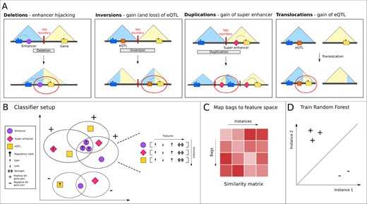
Overview of the steps in the svMIL method. (A) Rules applied by our model to link non-coding SVs to their effect on genes, and some biological examples of how these effects could be caused. (B) Each SV–gene pair is a bag, which contains instances representing regulatory elements. Each instance has its own feature vector. The number of features is the same between each instance, but each bag can have a different number and different types of instances. In this example, positive bags are identified by shared affected enhancers with a specific regulatory mark. (C) In the MILES approach, bags are mapped to a feature space by constructing a bag-to-instance similarity matrix. Positive bags will have smaller distances to positive instances than to negative instances, which (D) allows for a separation in feature space using a standard classifier
Deletions—If a deletion overlaps a TAD boundary, all genes in the TADs on either side of the deletion gain the regulatory elements from the TAD on the other side of the deletion.
Inversions—For inversions, genes lose regulatory elements that are inverted outside of the respective TAD, and gain elements that are inverted into the TAD. The genes residing in the inversion gain regulatory elements of the TAD that these genes are inverted into.
Duplications—If a duplication crosses a TAD boundary, it will generate a new TAD. Within this new TAD, genes in the duplication on the one side of the TAD boundary will be brought into contact with regulatory elements in the duplication on the other side of the TAD boundary.
Translocations—For each translocation independently, a derivative TAD is constructed based on the SV orientation. The gains and losses in the regulator set of every gene inside this new TAD are then determined.
Applying these rules results in a list of candidate SV–gene pairs and the associated gained and lost regulatory elements that are the result of the SV for this gene. To ensure that we are only looking at non-coding effects on genes, we removed SV–gene pairs for which the gene is overlapped (minimum 1 bp) by another SV, SNV or CNV in the same patient sample, as it is assumed that such coding events are the likely cause of any aberrant gene expression. As the affected genes can be overlapped by the respective SV itself, we make an exception for duplications and inversions (Fig. 1A). For inversions, we do not remove genes that are overlapped by the inversion when these are not affected by any other mutation. For duplications, we similarly keep the genes that are only overlapped by the duplication. As duplications often coincide with copy number (CN) amplifications (CN>2.3), we allow genes to be affected by such events only if these are also linked to a duplication by the rules.
2.3.3 Determining genes with altered expression
For each SV–gene pair, identified using the rules, we computed a z-score by comparing the expression of the gene in the patient with the SV to a null-distribution constructed based on all other patients (one-sample t-test). To ensure that the expression is changed by the non-coding SV specifically, we constructed the null-distribution only from patients that do not have an SNV, SV or CNV overlapping the gene. In addition, we removed potential non-coding effects from the null-distribution by excluding genes in patients where an SV disrupts the boundary of the TAD in which the gene is located. The z-scores are used as a measure of SV effect on the respective gene.
2.4 Step 2: machine learning to learn the characteristics of pathogenic SVs
To learn which SV–gene pair is likely pathogenic, and investigate if the gain or loss of specific regulatory elements are predictive for this, we trained a MIL model (Fig. 1B).
2.4.1 Defining bags and instances
Every SV–gene pair is considered a bag containing regulatory elements, the instances. The instances in each bag are defined as the regulatory elements lost or gained by the gene affected by the SV, as determined by the rules. We used a combination of eQTLs, enhancers and super enhancers as instances.
2.4.2 Instance features
Every instance is described with a feature vector combining three layers of features (Fig. 1B). The first layer consists of two features, indicating if the regulatory element is gained or lost. The second layer contains annotations of the region in which the regulatory element is located. This includes histone marks (H3K9me3, H3K4me3, H3K27ac, H3K27me3, H3K4me1, H3K36me3), chromHMM states (CTCF, CTCF+enhancer, CTCF+promoter, enhancer, promoter, poised promoter, heterochromatin, repeat, repressed, transcribed), transcription factor binding profiles (DNASeI hypersensitivity sites, RNA polymerase II, CTCF, transcription factor binding sites), CpG islands and Hi-C interacting regions. The feature vector contains a 0 or 1 depending on if the regulatory element overlaps any of these annotations (minimum 1 bp). Finally, we added a third layer to indicate the strength of the annotations. For enhancers, the prediction confidence score was used. For all histone marks, RNA polymerase II and CTCF, the peak intensity was used as an indicator of strength. This information was not available for any of the other annotations, and was thus left out. All features were normalized between 0 and 1.
2.4.3 Bag labels
We used the z-score of gene expression compared to unaffected TADs as a proxy for pathogenicity. Bags for SV–gene pairs with a z-score larger than 1.5 or smaller than -1.5 were labeled positive, and negative otherwise. To obtain equal class sizes, we randomly subsampled the negative bags to the same number of positive bags.
2.4.4 Multiple Instance Learning model
To obtain a final classifier, we used the MILES approach (Chen et al., 2006). One important feature of MILES is that it allows reconstructing which features of gained or lost regulatory elements are associated with positive SV–gene pairs. In MILES, the general idea is to map the bags to a feature space in which a standard classifier can be trained (Fig. 1C). This feature space is constructed by computing a similarity score between every bag and every instance. Positive bags are expected to be more similar to instances of other positive bags, but dissimilar to negative instances, therefore creating a separation in feature space (Fig. 1D). As all regulatory elements in each bag could equally contribute to the effect on gene expression, we compute the similarity score by first averaging the features of all instances in each bag, and then computing the absolute distance to all other instances of the other bags (collective assumption) (Carbonneau et al., 2018). A random forest is trained on the matrix of similarity scores to classify the SV–gene pairs. As the similarity matrix represents distances between bags as objects to instances as features, we used the random forest feature importance to rank individual instances.
2.4.5 Performance evaluation using cross-validation (CV)
We evaluate the model performance using three CV approaches. The first is a bag-based CV, in which bags are randomly distributed into the training and test set across 10 folds. To mimic a clinical setting, we use a leave-one-patient-out CV, in which all bags of one patient are held out in each fold. Lastly, we use a leave-one-chromosome-out CV, in which each chromosome is left out in every fold, to test for spatial correlation between SV–gene pairs. For each approach, in every fold one similarity matrix is constructed for the training bags, and one for the test bags, for which the similarity is computed to the instances of the training bags. Folds are stratified by randomly subsampling the number of negative bags to match the number of positive bags. The classifier was optimized using a random parameter search, applying 3-fold CV directly on the similarity matrix to reduce computational time.
3 Results
3.1 Altered gene expression is only visible in TADs disrupted by SVs
To show if SVs can affect gene expression by disrupting TADs and TAD boundaries, we compared the expression of genes in disrupted to non-disrupted TADs in the breast cancer patients. We define the TADs that an SV ends in on the left and right side as a ‘TAD pair’. We computed the z-score of gene expression inside these TAD pairs to all patients in which this pair is not disrupted by an SV, and filtered out mutated genes (see Section 2). As a negative control, we repeated this procedure for the TADs immediately to the left and right of each pair, keeping only adjacent TADs that are not disrupted by SVs in the respective patient. To account for varying TAD size, each TAD was divided into 10 bins. A minor increase in z-score is visible in the affected TADs, in particular for duplications and translocations (Fig. 2A). To determine if the gene expression is altered specifically by SVs and not due to effects such as methylation, we focused on all genes gaining or losing super enhancers as identified using the rules. Here also an overall increase in gene expression is visible (Fig. 2B), which is not observed when randomly shuffling the expression (Fig. 2C). Thus, we see that SVs are able to alter gene expression by re-shaping interactions between genes and regulatory elements.
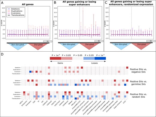
(A) The z-scores of all genes in disrupted TADs (right half) compared to the adjacent, non-disrupted TADs (left half), shown for each SV type. The two sides of the disrupted TAD pair, and the adjacent TADs on the left and right, were collapsed. The trend indicates the median z-score in each bin. Error bars indicate the 95th and 5th percentiles. (B) The z-scores shown specifically for genes that gain or lose super enhancers, as identified using the rules. (C) The z-scores shown in the same TADs as in (B), but when the gene expression is randomly shuffled. (D) Gains and losses of regulatory information that are significantly different between the positive set of SVs (effect on gene expression), negative set (no effect of gene expression), germline SVs, and when the positions of the positive SVs are shuffled randomly
3.2 Somatic SVs affect a unique combination of regulatory elements
To determine if SVs alter gene expression by affecting specific classes of regulatory elements, we compared their gain and loss patterns to those of SVs that do not affect expression (Fig. 2E, positive versus negative SVs). Overall, we observe significant differences for each SV type (P < 0.05, test with Bonferroni correction). These patterns are not observed when comparing to a case where the somatic SVs are assigned random positions (maintaining their size, type and chromosome), indicating that we do not find these differences by random chance (Fig. 2E, positive versus random SVs). Furthermore, the different gains and losses of regulatory elements observed when comparing to germline SVs suggest that somatic SVs occur at different genomic positions with different effects on regulatory elements (Fig. 2E, positive versus germline SVs). Taken together, these findings indicate that disrupted interactions with regulatory elements contain information on the pathogenicity of somatic SVs.
3.3 svMIL can successfully identify pathogenic SVs in various cancer types
To determine if re-wiring patterns are informative predictors of pathogenicity, we trained MIL models with a random forest classifier to separate SV–gene pairs with large effects on gene expression from SV–gene pairs with no effects (Section 2). A model was trained on each SV type individually, using the same number of bags in each class (deletions: 168, duplications: 906, inversions: 338 and translocations: 133).
To mimic a clinical setting, in which prioritization of the SVs in the cancer genome of a new and unseen patient is required, we performed leave-one-patient-out CV. We find that svMIL can successfully identify pathogenic SVs in unseen patients with AUCs of 0.79, 0.66, 0.78 and 0.82 for deletions, duplications, inversions and translocations, respectively (Fig. 3A). Notably, such classification performance is not observed when the SV positions are shuffled randomly (Supplementary Fig. S2A). Thus, our method is suitable to predict pathogenic SVs in clinical settings.
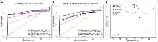
ROC curves based on leave-one-patient out CV for the models trained on each SV type for (A) the HMF BRCA dataset and (B) the PCAWG ovarian cancer dataset. (C) The TPR and FPR of svMIL compared to three other methods. svMIL is highlighted by the dotted oval
As a note of warning, bag-based CV, which is the classical CV strategy, yields much higher performances (Supplementary Fig. S2B). However, we observed that patients frequently have multiple spatially clustered SVs affecting the same gene, causing gains and losses of the same instances. Since these pairs are randomly distributed across the training and test set in each fold, this may cause some information leakage and biased CV results. Indeed, when validating our model in a per-chromosome CV setting, similar results were obtained to the leave-one-patient-out CV (Supplementary Fig. S2C). A similar issue could arise in the leave-one-patient-out CV if many SVs are shared between multiple patients. Therefore, caution is advised when interpreting results of bag-based CV or leave-one-patient-out CV settings in these situations.
Furthermore, we realize that our P-value threshold for eQTLs of P< is especially stringent, and that lowering the threshold to P < 0.05 improves the AUC for deletions to 0.88. However, due to the sheer increase in the number of eQTLs, lowering the threshold increases the run time to up to 24 h for deletions alone, and is therefore not realistic to run in routine analysis. Nevertheless, these results reveal potential for further improvement in predictive ability.
Finally, we aimed to demonstrate the performance in other cancers. To this end, we retrained svMIL on ovarian cancer samples from the PCAWG dataset. Notably, the number of bags is slightly larger than for our breast cancer dataset (deletions: 256, duplications: 1009, inversions: 818, translocations: 229). Nevertheless, the ROC curves demonstrate that also for ovarian cancer, similar performances are obtained (Fig. 3B), indicating that our method is applicable to various cancer types.
3.4 svMIL outperforms the state-of-the-art methods
Next, we aimed to show how our method compares to the state-of-the-art. We compared the true positive rate (TPR) and false positive rate (FPR) of our method to VEP, SVScore and a random forest classifier without MIL (non-MIL-RF). For VEP, SVs with a ’moderate’ or ’high’ impact score were considered pathogenic. For SVScore, pathogenic SVs were selected using scores above the 90th percentile (for each SV type separately). For the non-MIL-RF, we used gains and losses of regulatory elements of each SV–gene pair as binary features. If multiple regulatory elements of a type are affected, the feature value was capped at 1. We used an operating point of 0.5 for both svMIL and non-MIL-RF and tested performance using leave-one-patient-out CV. For each method, an SV is considered positive if it is part of a positive SV–gene pair.
Overall, we see that svMIL obtains higher TPR than the other methods when predicting SV pathogenicity in unseen patients (Fig. 3C). Non-MIL-RF also scores high TPR, but at a cost of increased FPR compared to svMIL, showing the benefit of identifying pathogenic SVs using a MIL-based approach. VEP and SVScore both score low FPR, but also never have TPR above 0.1. As both methods do not include TAD disruptions or gene expression in their predictions, these results show that performance can be improved if such additional data layers are integrated.
3.5 SVs frequently re-wire active (super) enhancers in open chromatin regions
Using our trained MIL classifiers, we investigated which regulatory elements are most commonly associated with pathogenic SVs. We obtained a ranked list of instances for each MIL model from the random forest feature importance scores. As a threshold, we focused on the top 100 instances of each model, which retains the majority of information for each SV type (Supplementary Fig. S3). Overall, we find that the affected regulatory elements are significantly associated with open chromatin regions and histone marks enriched in active promoters and enhancers (compared to 100 randomly sampled instances, P < 0.05, Bonferroni) (Fig. 4A). Each SV type affects a unique set of regulatory elements. For instance, deletions and duplications frequently cause gains of active enhancers, while inversions and translocations instead more often result in gains and losses of super enhancers, revealing a possible different mechanism by which target genes are affected. We furthermore note that the majority of top-ranked instances are gains rather than losses (89/100 and 58/100 gains for inversions and translocations, respectively), indicating that gains of regulatory elements could be a preferred method to affect gene expression in breast cancer.
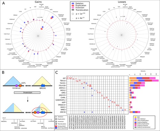
(A) Gains and losses in the top 100 instances per SV type. Values above the red dotted lines are significant (P < 0.05, Bonferroni) with a z-score larger than 0 (more than in 100 randomly selected instances), values below the red dotted line with a z-score smaller than 0 (less than in 100 randomly selected instances). Everything within the red dotted lines is not significant. (B) Inversion bringing enhancers and eQTLs from another TAD close to BRCA1, resulting in overexpression. For simplicity, only one enhancer and one eQTL is shown. (C) Top 15 genes most recurrently affected across patients by SVs within the top 100 instances of each SV type. Only patients with positive SV–gene pairs are included in the analysis. The bars show the number of patients with a coding mutation overlapping that same gene. Some patients have multiple mutations
To determine if the gains and losses could potentially be causal for cancer, we compared the instances within the ranked top 100 that affect known cancer genes (COSMIC genes; 5, 5, 1 and 4 out of 100 instances for deletions, duplications, inversions and translocations, respectively) to those affecting non-COSMIC genes (Supplementary Fig. S4). Overall, we see that COSMIC genes and non-COSMIC genes show similar patterns, indicating a potential similar effect on genes. Taken together, these findings suggest that our ranking can successfully identify pathogenic mechanisms of SVs and bona fide target genes of SVs.
3.6 svMIL can identify driver genes in unseen patients
Motivated by the similarities in gained and lost regulatory elements between known cancer genes and other genes, we investigated if our method can identify potential novel driver genes. To this end, we employed leave-one-patient-out CV, specifically for the patients with an SV linked to a known COSMIC gene. This enabled us to determine how often a known COSMIC gene is correctly classified as pathogenic, using a classifier trained on data that has never seen this SV–gene pair. In total, 34 (out of 64) SV-COSMIC gene pairs were predicted correctly, which are significantly more COSMIC genes than expected by random chance (P = 3.86e-172, t-test, compared to 100 iterations of leave-one-patient-out CV where random SV–gene pairs were assigned to the bags after the classification step). For none of these COSMIC genes there was any other evidence, such as SNVs or indels, that could have disrupted it, which means it would not have been identified otherwise. Notably, four of these SV–gene pairs identified genes specific to breast cancer (one inversion targeting BRCA1, and three duplications targeting ERBB2 in the same patient). Of particular interest is the inversion affecting BRCA1, bringing 3 enhancers and 46 eQTLs in close proximity to the gene (Fig. 4B). High BRCA1 expression has previously been linked to worse prognosis in several cancers, including breast cancer, and could therefore be an interesting finding for selecting treatment (He et al., 2015; Wang et al., 2018a). In addition, BRCA1 is upregulated in 11.4% of breast cancer patients (CGC), indicating that this SV could be an alternative pathway to upregulate the gene (Tate et al., 2019). Altogether, these results demonstrate the importance of incorporating non-coding SVs in the analysis of whole cancer genome sequencing data of patients.
In addition, we investigated if genes linked to high-ranking SVs are recurrently affected (z > 1.5 or z < -1.5) across different patients by other non-coding SVs, and could therefore be putative cancer drivers. We obtained the genes from the top 100 ranked instances of all SV types, and report the top 15 most recurrently mutated in Figure 4C. Some patients have multiple non-coding SVs targeting the same gene, indicative of selective pressure. Most genes affected by deletions and duplications are only upregulated in their respective patients, while we see both up- and downregulation for inversions and translocations, showing that the majority of SVs can indeed be responsible for the gene expression change. Moreover, we identify a large number of SNVs, CNVs and coding SVs targeting the same gene in other patients, showing that non-coding SVs could be an alternative route to affect important genes in the cancer genome.
Finally, we note that the number of patients in which the top 15 genes are recurrently affected is not significant (P < 0.05, Bonferroni, compared to 100 distributions of randomly sampled positive SV–gene pairs) and appears to be much smaller than for other mutation types, which has also been reported previously (Rheinbay et al., 2020). In addition, we identify different recurrently affected genes if we do not filter by the top-ranked instances (Supplementary Fig. S5), supporting the importance of applying machine learning-based methods to identify pathogenic SVs, and including gene expression into these models.
4 Discussion
In this work, we described svMIL, a novel MIL-based method to rank SVs for their likelihood to be pathogenic based on altering interactions between genes and regulatory elements and thereby disrupting gene expression. Not all genes in disrupted TADs show affected expression levels. However, the genes that are affected can be pinpointed by looking at gains and losses of regulatory elements caused by SVs. Using our MIL model, we can now utilize this information to identify pathogenic SVs in various cancer types. We demonstrated, by mimicking a clinical setting using leave-one-patient-out CV, that svMIL can successfully identify pathogenic SVs in unseen patients. Within these unseen patients, we identified SVs affecting known cancer genes that were not disrupted by any other mutations, such as SNVs, thus revealing the importance of also studying non-coding SVs in clinical analyses. As such methods to predict the effect of non-coding SVs are currently lacking, our model provides an opportunity to study existing and future SV datasets in more detail.
We showed that top-ranking pathogenic SVs frequently affect active (super) enhancers in open chromatin regions. Furthermore, regulatory elements are more frequently gained than lost in the breast cancer samples, showing a possible preference to upregulate genes in these patients. Many genes disrupted by top-ranking pathogenic SVs are recurrently affected by non-coding SVs across multiple patients, with frequent evidence of other mutations, such as CNVs, disrupting the same genes. These findings show that non-coding SVs could be an important alternative strategy to disrupt genes that are important in cancer cells. As these same genes could not be identified independent of the ranking by pathogenicity produced by svMIL, it highlights the benefit of utilizing gene expression information and MIL models to identify pathogenic SVs.
As more and more data are becoming available for cancer patients, our ability to predict pathogenicity will continue to improve. For example, the absence of methylation and 3D folding data for each patient limits our ability to perfectly label which genes are truly affected by the SV only. Additionally, an increase in cell-type specific and validated regulatory elements will make it possible to further fine-tune predictive models.
Nevertheless, our presented model can aid in understanding the consequences of SVs in more detail, allowing the generation of new hypotheses about the role of SVs in cancer.
Data availability
The WGS and RNA-seq breast cancer data were requested from the Hartwig Medical Foundation and provided under data request DR-066.
Financial Support: none declared.
Conflict of Interest: none declared.

