Conditional out-of-distribution generation for unpaired data using transfer VAE Free

Abstract

1 Introduction

The task of generating high-dimensional samples x conditional on a latent random vector z and a categorical variable s has established solutions (Mirza and Osindero, 2014; Ren et al., 2016). The situation becomes more complicated if the support of z is divided into domains d that come with different meanings: say $d∈{cat,dog}$ and one is interested in out-of-distribution (OOD) generation of samples x in a domain and condition (d, s) that are not part of the training data. Now, predicting how a given brown dog would look like with black fur becomes an OOD problem if the training data does not have observations of black dogs. To still have a chance of solving it, we assume training data with brown dogs, and brown and black cats. In an application with higher relevance, there is strong interest in how untreated humans (⁠$s=0,d=0$⁠) respond to drug treatment (s = 1) based on training data from human in vitro (d = 1) and in vivo mouse (d = 2) experiments. Hence, the target domain of interest (d = 0) does not offer training data for s = 1, but only for s = 0.

In this article, we suggest to address the challenge of generating samples OOD by regularizing the joint distribution across the categorical variable s using maximum mean discrepancy (MMD) in the framework of a conditional variational autoencoder (CVAE) (Sohn et al., 2015). This produces a more compact representation of a cross-condition distribution that would otherwise display high variance in the standard CVAE. We will show that this leads to more accurate OOD prediction. MMD has proven successful in a variety of tasks. In particular, matching distributions with MMD in variational autoencoders (VAEs) (Kingma and Welling, 2013) has been suggested for unsupervised domain adaptation (Louizos et al., 2015) or for learning statistically independent latent dimensions (Lopez et al., 2018b). In supervised domain adaptation approaches, MMD-based regularization has been shown to be a viable strategy of learning label-predictive features that are stripped off of domain-specific information (Long et al., 2015; Tzeng et al., 2014). In these instances, however, MMD was used at the bottleneck layer, where it leads to different properties.

Matching distributions across perturbed and control populations has also been studied in the context of causal inference (Johansson et al., 2016), albeit not in the context of generative modeling and OOD generation. Johansson et al. (2016) showed how to improve counterfactual inference by learning representations that enforce similarity between perturbed and control using a linear discrepancy measure, mentioning MMD as an alternative metric.

In further related work, the OOD generation problem was addressed via hard-coded latent space vector arithmetics (Lotfollahi et al., 2019) and histogram matching (Amodio et al., 2018). The approach of this article, however, introduces a data-driven end-to-end approach, which does not involve hard-coded elements and generalizes to more than one condition. We hope this work further stimulates the recent success of generative models in single-cell biology (Eraslan et al., 2019; Lopez et al., 2018a).

2 Materials and methods

2.1 Variational autoencoder

The right hand side of this equation provides the cost function $ℓVAE$ for optimizing neural-network based parametrizations of $pθ$ and $qϕ$⁠. The left-hand side describes the likelihood subtracted by an error term.

The case in which $S≠ϕ$ is referred to as the CVAE (Sohn et al., 2015), and a straight-forward extension of the original framework (Kingma and Welling, 2013), which treated $S≡ϕ$⁠.

2.2 Maximum-mean discrepancy

In contrast to GANs (Goodfellow et al., 2014) whose training procedure is notoriously hard due to the minmax optimization problem, training models using MMD or Wasserstein distance metrics is comparatively simple (Arjovsky et al., 2017; Dziugaite et al., 2015a; Li et al., 2015) as only a direct minimization of a single loss is involved. It has been shown that MMD-based GANs have some advantages over Wasserstein GANs resulting in a simpler and faster-training algorithm with matching performance (Bińkowski et al., 2018). This motivated us to choose MMD as a metric for implementing distribution matching as a regularization of a CVAE.

2.3 Transfer VAE

Fig. 1.

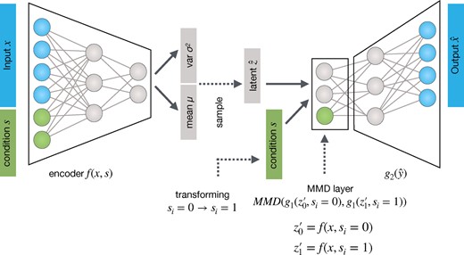
Transfer VAE (trVAE) is an MMD-regularized conditional VAE. It receives randomized batches of data (x) and condition (s) as input during training, stratified for approximately equal proportions of s. In contrast to a standard CVAE, we regularize the effect of s on the representation obtained after the first-layer $g1(z^,s)$ of the decoder g. During prediction time, we transform batches of the source condition $xs=0$ to the target condition $xs=1$ by encoding $z^0=f(x0,s=0)$ and decoding $g(z^0,s=1)$

Open in new tabDownload slide

However, even if z is completely free of variation from s, the y representation has a strong s component, $Y⊥⊥S$⁠, which leads to a separation of $ys=1$ and $ys=0$ into different regions of their support $Y$⁠. In the standard CVAE, without any regularization of this y representation, a highly varying, non-compact distribution emerges across different values of s (Fig. 2). To compactify the distribution so that it displays only subtle, controlled differences, we impose MMD Equation 2 in the first layer of the decoder (Fig. 1). We assume that modeling y in the same region of the support of $Y$ across s forces learning common features across s where possible. The more of these common features are learned, the more accurately the transformation task will performed and the higher are chances of successful OOD generation. Using one of the benchmark datasets introduced, below, we qualitatively illustrate the effect (Fig. 2).

Fig. 2.

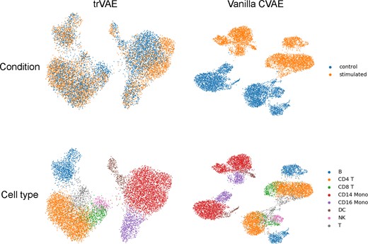
Comparison of representations for MMD-layer in trVAE and the corresponding layer in the standard CVAE using UMAP (McInnes et al., 2018). The MMD regularization incentivizes the model to learn condition-invariant features resulting in a more compact representation. The figure shows the qualitative effect for the ‘PBMC data’ introduced in experiments section. Both representations show the same number of samples

Open in new tabDownload slide

During training time, all samples are passed to the model with their corresponding condition labels $(xs,s)$⁠. At prediction time, we pass $(xs=0,s=0)$ to the encoder f to obtain the latent representation $z^s=0$⁠. In the decoder g, we pass $(z^s=0,s=1)$ and through that, let the model transform data to $x^s=1$⁠.

4 Results

We demonstrate the advantages of an MMD-regularized first layer of the decoder by benchmarking versus a variety of existing methods and alternatives:

• Standard CVAE (Sohn et al., 2015)

• CVAE with MMD on bottleneck (MMD-CVAE), similar to VFAE (Louizos et al., 2015)

• MMD-regularized autoencoder (Amodio et al., 2019; Dziugaite et al., 2015b)

• CycleGAN (Zhu et al., 2017)

• scGen, a VAE combined with vector arithmetics (Lotfollahi et al., 2019)

• scVI, a CVAE with a negative binomial output distribution (Lopez et al., 2018a).

First, we demonstrate trVAE’s basic OOD style transfer capacity on two established image datasets, on a qualitative level. We then address quantitative comparisons of challenging benchmarks with clear ground truth, predicting the effects of biological perturbation based on high-dimensional structured data. We used convolutional layers for imaging examples in section and fully connected layers for single-cell gene expression datasets in sections and. The optimal hyper-parameters for each application were chosen by using a parameter gird-search for each model.

4.1 MNIST and CelebA style transformation

Here, we use Morpho-MNIST (Castro et al., 2018), which contains 60 000 images each of ‘normal’ and ‘transformed’ digits, which are drawn with a thinner and thicker stroke. For training, we used all normal-stroke data. Hence, the training data covers all domains (⁠$d∈{0,1,2,…,9}$⁠) in the normal stroke condition (s = 0). In the transformed conditions (thin and thick strokes, $s∈{1,2}$⁠), we only kept domains $d∈{1,3,6,7}$⁠.

We train a convolutional trVAE in which we first encode the stroke width via two fully connected layers with 128 and 784 features, respectively. Next, we reshape the 784-dimensional into 28*28*1 images and add them as another channel in the image. Such trained trVAE faithfully transforms digits of normal stroke to digits of thin and thicker stroke to the OOD domains (Fig. 3).

Fig. 3.

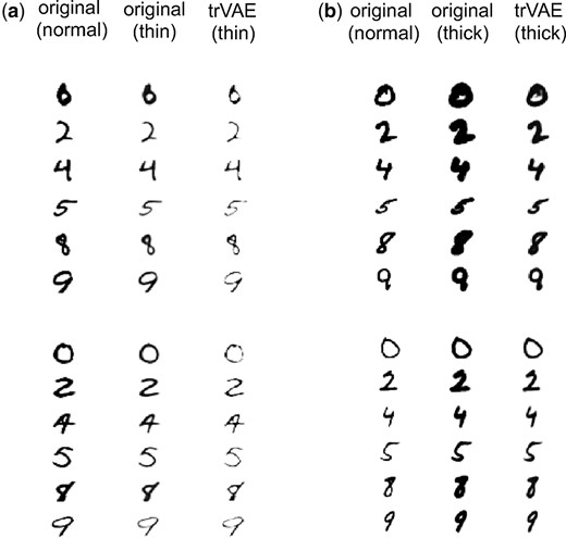
OOD style transfer for Morpho-MNIST dataset containing normal, thin and thick digits. trVAE successfully transforms normal digits to thin (a) and thick (b) for digits not seen during training (OOD)

Open in new tabDownload slide

Next, we apply trVAE to CelebA (Liu et al., 2015), which contains 202 599 images of celebrity faces with 40 binary attributes for each image. We focus on the task of learning a transformation that turns a non-smiling face into a smiling face. We kept the smiling (s) and gender (d) attributes and trained the model with images from both smiling and non-smiling men but only with non-smiling women.

In this case, we trained a deep convolutional trVAE with a U-Net-like architecture (Ronneberger et al., 2015). We encoded the binary condition labels as in the Morpho-MNIST example and fed them as an additional channel in the input.

Predicting OOD, trVAE successfully transforms non-smiling faces of women to smiling faces while preserving most aspects of the original image (Fig. 4). In addition to showing the model’s capacity to handle more complex data, this example demonstrates the flexibility of the model adapting to well-known architectures like U-Net in the field.

Fig. 4.

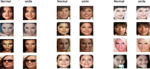
CelebA dataset with images in two conditions: celebrities without a smile and with a smile on their face. trVAE successfully adds a smile on faces of women without a smile despite these samples completely lacking from the training data (OOD). The training data only comprises non-smiling women and smiling and non-smiling men

Open in new tabDownload slide

4.2 Infection response

Accurately modeling cell response to perturbations is a key question in computational biology. Recently, neural network models have been proposed for OOD predictions of high-dimensional tabular data that quantifies gene expression of single-cells (Amodio et al., 2018; Lotfollahi et al., 2019). However, these models are not trained on the task relying instead on hard-coded transformations and cannot handle more than two conditions.

We evaluate trVAE on a single-cell gene expression dataset that characterizes the gut (Haber et al., 2017) after Salmonella or Heligmosomoides polygyrus (H. poly) infections, respectively. For this, we closely follow the benchmark as introduced in Lotfollahi et al. (2019). The dataset contains eight different cell types in four conditions: control or healthy cells (n = 3240), H.Poly infection a after three days (H.Poly.Day3, n = 2121), H.poly infection after 10 days (H.Poly.Day10, n = 2711) and salmonella infection (n = 1770) (Fig. 5a). The normalized gene expression data has 1000 dimensions corresponding to 1000 genes. Since three of the benchmark models are only able to handle two conditions, we only included the control and H.Poly.Day10 conditions for model comparisons. In this setting, we hold out Tuft infected cells for training and validation, as these constitute the hardest case for OOD generalization (least shared features, few training data).

Fig. 5.

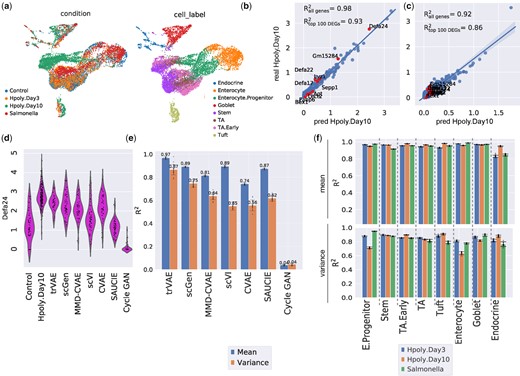
(a) UMAP visualization of conditions and cell type for gut cells. (b and c) Mean and variance expression of 1000 genes comparing trVAE-predicted and real infected Tuft cells together with the top 10 differentially expressed genes highlighted in red (R² denotes Pearson correlation between ground truth and predicted values). (d) Distribution of Defa24: the top response gene to H.poly.Day10 infection between control, predicted and real stimulated cells for different models. Vertical axis: expression distribution for Defa24. Horizontal axis: control, real and predicted distribution by different models. (e) Comparison of Pearson’s R² values for mean and variance gene expression between real and predicted cells for different models. Center values show the mean of R² values estimated using n = 100 random subsamples for the prediction of each model and error bars depict standard deviation. (f) Comparison of R² values for mean and variance gene expression between real and predicted cells by trVAE for the eight different cell types and three conditions. Center values show the mean of R² values estimated using n = 100 random subsamples for each cell type and error bars depict standard deviation

Open in new tabDownload slide

Figure 5b and c shows trVAE accurately predicts the mean and variance for high-dimensional gene expression in Tuft cells. We compared the distribution of Defa24, the gene with the highest change after H.poly infection in Tuft cells, which shows trVAE provides better estimates for mean and variance compared to other models. Moreover, trVAE outperforms other models also when quantifying the correlation of the predicted 1000 dimensional x with its ground truth (Fig. 5e). In particular, we note that the MMD regularization on the bottleneck layer of the CVAE does not improve performance, as argued above.

In contrast to existing approaches, trVAE can handle multiple perturbations at the same time. To illustrate this, we performed another experiment by training eight different models holding out each of the eight cell types form all three conditions. trVAE accurately predicts all cell types across different perturbations (Fig. 5f). The ability to handle multiple perturbations enables analysis and prediction for large drug screening studies.

4.3 Stimulation response

Similar to modeling infection response as above, we benchmark on another single-cell gene expression dataset consisting of 7217 IFN-β stimulated and 6359 control peripheral blood mononuclear cells (PBMCs) from eight different human Lupus patients (Kang et al., 2018). The stimulation with IFN-β induces dramatic changes in the transcriptional profiles of immune cells, which causes big shifts between control and stimulated cells (Fig. 6a). We studied the OOD prediction of natural killer (NK) cells held out during the training of the model.

Fig. 6.

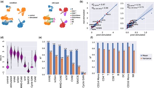
(a) UMAP visualization of peripheral blood mononuclear cells (PBMCs). (b and c) Mean and variance per 2000 dimensions between trVAE-predicted and real natural killer cells (NK) together with the top 10 differentially expressed genes highlighted in red. (d) Distribution of ISG15: the most strongly changing gene after IFN-β perturbation among control, real and predicted stimulated cells for different models. Vertical axis: expression distribution for ISG15. Horizontal axis: control, real and predicted distribution by different models. (e) Comparison of R² values for mean and variance gene expression between real and predicted cells for different models. Center values show the mean of R² values estimated using n = 100 random subsamples for the prediction of each model and error bars depict standard deviation. (f) Comparison of R² values for mean and variance gene expression between real and predicted cells by trVAE for eight different cells in the study. Center values show the mean of R² values estimated using n = 100 random subsamples for each cell type and error bars depict standard deviation

Open in new tabDownload slide

trVAE accurately predicts mean (Fig. 6b) and variance (Fig. 6c) for all genes in the held out NK cells. In particular, genes strongly responding to IFN-β (highlighted in red in Fig. 6b and c) are well captured. An effect of applying IFN-β is an increase in ISG15 for NK cells, which the model never sees during training. trVAE predicts this change by increasing the expression of ISG15 as observed in real NK cells (Fig. 6d). A cycle GAN and an MMD-regularized auto-encoder (SAUCIE) and other models yield less accurate results than our model. Comparing the correlation of predicted mean and variance of gene expression for all dimensions of the data, we find trVAE performs best (Fig. 6e). To demonstrate the generality of our method we trained seven other models, removing stimulated cells for each of seven different cell types in the study. Our model robustly predicted all other seven cell types (Fig. 6f).

The specificity of perturbation responses of cells depends on many factors leading to changes in gene expression levels that are either shared across all types or specific to some. Predicting both groups of responses is necessary to address questions such as which cell types are most responsive to a perturbation, and successful drug dose prediction (Hu et al., 2020; Srivatsan et al., 2020).

trVAE can capture specific responses after IFN-β when any of the cell types is absent from training and afterward predicted. To demonstrate this, we scored the specificity of differently expressed genes (DEGs) after IFN-β stimulation using a median-based score (see Supplementary Methods). trVAE successfully predicts top 10 most cell-type-specific responding genes (Fig. 7a). Specifically, our model predicted the up-regulation of CCL8, a CD14-Mono specific response gene after IFN-β. As another example, trVAE not only predicted the up-regulation of ISG15 as a shared response gene but also captured the specific expression pattern of this gene across different cell types. Next, we compared our approach with the state-of-the-art model (scGen) for this task using the top 250 most cell-type-specific DEGs. Our model improves the mean error on the first and the second top 50 specific DEGs by 65% and 44%, respectively (Fig. 7b and c). Further comparison demonstrated that trVAE not only outperforms scGen but also all other benchmarked methods (Supplementary Figs S1 and S2).

Fig. 7.

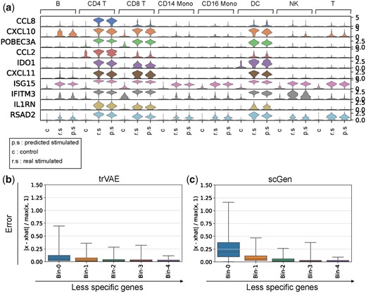
(a) Violin plot for top 10 specific response genes after IFN-β stimulation out of 250 DEGs according to the gene specificity score across control (c), real stimulated (r.s) and predicted stimulated (p.s) for different cell types. Vertical axis: expression distribution for top specific genes. Horizontal axis: control, real and predicted distribution by trVAE for different cell types. (b and c) Box plots of top 500 DEGs ordered by the gene specificity score. Each bin is composed of 50 genes and each point in the bin shows the error between average expression of that gene within a cell type and average prediction by trVAE and scGen for that cell type. In total, each boxplot has been derived from 50 (number of genes)×8 (number of cell types) points (n = 400). Box plots indicate the median (center lines), interquartile range (hinges) and whiskers represents min and max values

Open in new tabDownload slide

5 Discussion

By arguing that the standard CVAE yields representations in the first layer following the bottleneck that vary strongly across categorical conditions, we introduced an MMD regularization that forces these representations to be similar across conditions. The resulting model (trVAE) outperforms existing modeling approaches on benchmark and real-world datasets.

Within the bottleneck layer, CVAEs already display a well-controlled behavior and regularization does not improve performance. Further regularization at later layers might be beneficial but is numerically costly and unstable as representations become high-dimensional. However, we have not yet systematically investigated this and leave it for future studies.

We have evaluated the predictive power of trVAE by leaving out one cell type and trying to predict it in cases in which the training data contains cell types that are rather similar to the targeted OOD cells (Lotfollahi et al., 2019). Further evaluation is needed when OOD samples are very different from the training data. Also, further studies are required to understand the uncertainty quantification inherent to the probabilistic nature of the model. Finally, we note that architectures related to Gaussian mixture VAEs or GANs may be considered as alternatives to the MMD regularization.

The ability to analyze and predict multiple perturbations allow trVAE to be applied to experiments with many biological conditions. Specifically, recent advances in massive single-cell compounds screening (Srivatsan et al., 2020) provide great potential to exploit our model for further experimental design and the study of interaction effects among different drugs. Future conceptual investigations concern establishing connections to causal-inference-inspired models beyond (Johansson et al., 2016) such as CEVAE (Louizos et al., 2017), establishing further that faithful modeling of an interventional distribution can be re-framed as successful perturbation effect prediction across domains.

Acknowledgements

The authors are grateful to Anna Klimovskaia for pointing us to the reference of Johansson et al. (2016) and to Romain Lopez for pointing us to problems with the background section on the VAE in the arXiv preprint version of this manuscript.

Financial Support: This work was supported by BMBF grant nos. 01IS18036A and 01IS18053A, by the German Research Foundation within the Collaborative Research Center 1243, Subproject A17, by the Helmholtz Association (Incubator grant sparse2big, grant no. ZT-I-0007) and by the Chan Zuckerberg Initiative DAF (advised fund of Silicon Valley Community Foundation, no. 182835). M.L. acknowledges financial support from the Joachim Herz Stiftung.

Conflict of Interest: F.J.T. reports receiving consulting fees from Roche Diagnostics GmbH and Cellarity Inc., and ownership interest in Cellarity, Inc. F.A.W. reports being a full-time employee of Cellarity Inc., and ownership interest in Cellarity, Inc.

Data availability

All of the data sets analyzed in this manuscript are public and published in other papers. We have referenced them in the manuscript and they are downloadable at github.com/theislab/trvae_reproducibility.

References