ARMBIS: accurate and robust matching of brain image sequences from multiple modal imaging techniques

Abstract

Motivation

Study of brain images of rodent animals is the most straightforward way to understand brain functions and neural basis of physiological functions. An important step in brain image analysis is to precisely assign signal labels to specified brain regions through matching brain images to standardized brain reference atlases. However, no significant effort has been made to match different types of brain images to atlas images due to influence of artifact operation during slice preparation, relatively low resolution of images and large structural variations in individual brains.

Results

In this study, we develop a novel image sequence matching procedure, termed accurate and robust matching brain image sequences (ARMBIS), to match brain image sequences to established atlas image sequences. First, for a given query image sequence a scaling factor is estimated to match a reference image sequence by a curve fitting algorithm based on geometric features. Then, the texture features as well as the scale and rotation invariant shape features are extracted, and a dynamic programming-based procedure is designed to select optimal image subsequences. Finally, a hierarchical decision approach is employed to find the best matched subsequence using regional textures. Our simulation studies show that ARMBIS is effective and robust to image deformations such as linear or non-linear scaling, 2D or 3D rotations, tissue tear and tissue loss. We demonstrate the superior performance of ARMBIS on three types of brain images including magnetic resonance imaging, mCherry with 4′,6-diamidino-2-phenylindole (DAPI) staining and green fluorescent protein without DAPI staining images.

Availability and implementation

The R software package is freely available at https://www.synapse.org/#!Synapse:syn18638510/wiki/591054 for Not-For-Profit Institutions. If you are a For-Profit Institution, please contact the corresponding author.

Supplementary information

Supplementary data are available at Bioinformatics online.

1 Introduction

Brain research has been significantly facilitated in the past several years due to the launch of several brain projects in Europe, USA, Japan and Korea (Poo et al., 2016). For these brain projects, rodent animals play a very important role for a large number of shared genes with human and easy operation of genome editing. Brain images are important for studying the brain functions or the neural basis of physiological functions (Toga, 2015).

Brain imaging can be done invasively or non-invasively. Non-invasive in vivo methods include positron emission tomography (PET) and magnetic resonance imaging (MRI) while brain slices imaging with histology or other technologies obtained with various microscopes are typical invasive approaches. For those brain images, it is important to visualize and explore them against standardized brain reference atlases and the very first step is to find the best matched atlas image for a query brain image (Ng et al., 2012). However, due to influence of artifact operation during slice preparation (e.g. tissue folds, tears, regions missing, tissue stretch or compress), variations in sample structures or damaged regions, precise matching is usually very difficult and thus the matching procedure is usually performed manually in most neuroanatomical laboratories, and (Agarwal et al., 2016; Yushkevich et al., 2006). Recently, Agarwal (Agarwal et al., 2017) and Midroit (Midroit et al., 2018) developed two methods to align histological sections and achieved some promising results. However, these methods do not have the function for matching brain slices.

To our knowledge, no method has been developed to match different kinds of brain images (e.g. matching MRI images to the atlas images) due to several challenges. First, query images and atlas images cannot be directly compared as they are likely to have different scales (sizes). Different scales between query images and atlas images are one key factor affecting the matching performance especially when image textures are used. Second, the relative low spatial resolution and image contrast as well as large structural variations pose a great challenge for feature-based image matching. Even some scale invariant features such as SIFT (Scale Invariant Feature Transform) (Lowe, 2004) cannot work well under such situations (Wu et al., 2009). Third, image sequence matching has to take into account large variations, due to different resolutions or artifacts during sample slicing, between query images and atlas images which may lead to unevenly spaced atlas images.

In this study, we developed a novel effective image-sequence matching framework, termed accurate and robust matching of brain image sequences (ARMBIS), to match query image sequences to reference brain image atlases (Fig. 1). To take advantage of the spatial relationship among 3D image slices in both test and atlas image sequences, the change rates of the geometric features extracted from image sequences are used to first estimate a scaling factor and then roughly locate the query image sequence in the atlas image sequence. Then the query images are rescaled by the estimated scaling factor so that the two image sequences are comparable in size and suitable for exact matching based on texture and shape features. The global texture similarity is measured by mutual information of the overall local binary pattern (LBP) while the local similarity is measured by the intersection distance of the corresponding regional LBP histograms. In addition to these texture features, scale and rotation invariant shape features are extracted as well. Then, a mathematical induction-based optimization under the constraints of order and distance for the best matched indices is implemented to the grouped global texture and shape features to identify several optimal subsequences. Finally, the best matched subsequence in the atlas images is determined by a hierarchical decision approach using local texture features.

Fig. 1.

The architecture of ARMBIS for matching image sequences. ARMBIS takes a query image sequence and an atlas image sequence as inputs and outputs the best matched image sequence in the atlas. (A) Extraction of shape features. (B) Break point detection and curve fitting. Left: the original feature curve of the atlas image sequence (blue line) represented by piecewise linear (black dotted line) divided by several break points (red triangle). Middle: The original feature curve of the query image sequence (orange line) represented piecewise linear (black dotted line) divided by several break points (purple triangle). Right: Matching the two curves by matching two slope sequences. (C) Extraction of texture features. (D) Feature fusion and feature enhancement for fused similarity curve (⁠ ${Sim}_{i}^{feature}$ ⁠) of each query image. First all the spikes are identified as $d ({Sim}_{i}^{feature}) < 0$ and then the spikes greater than the mean of ${Sim}_{i}^{feature}$ (gray dotted line) and their eight nearest neighbors are selected as candidate peaks. Finally the values on the candidate peaks are scaled up by a constant $c$ (c $> 1)$ ⁠. (E) The optimization procedure based on the fused similarity matrix $Sim$ ⁠. The orange squares indicate the selected indices in each row which leads to maximal $\sum_{j = 1}^{N} {Sim}_{j, mj}$ ⁠. The intervals between adjacent indices of $m$ are within the range of $[c - g, c + g]$ ⁠. (F) A hierarchical decision procedure identifies the final best matched atlas images by local texture features. The ranking of each optimal matching patch is obtained by Equation (9). (G) Output of the best matched image sequence in atlas

Open in new tab Download slide

The rest of the paper is organized as follows. Section 2 introduces ARMBIS in detail. Section 3 evaluates the performance of our proposed method using simulation data and real brain MRI data. Section 4 concludes the article.

2 Methods

Given a sequence of query images $I^{T} = [I_{1}^{T}, I_{2}^{T}, \dots, I_{N}^{T}]$ and a sequence of atlas images $I^{A} = [I_{1}^{A}, I_{2}^{A}, \dots, I_{K}^{A}]$ ⁠, the goal is to match each individual query image $I_{j}^{T}$ (⁠ $j = 1, 2, \dots, N$ ⁠) to an atlas image $I_{m_{j}}^{A} {(m}_{j} \in {1, 2, \dots, K}$ ⁠), where $m_{j}$ is the index of the best matched atlas image for a query image $j$ ⁠, and the best matched indices are under the constraint of $m_{j - 1} < m_{j} < m_{j + 1}$ or $m_{j - 1} > m_{j} > m_{j + 1}$ ⁠.

2.1 Feature extraction

Feature extraction is the most important step in pattern matching. In the proposed method, texture and shape features are extracted, as described in Figure 1A–C, and the flowchart of the detailed feature extraction procedure is given in Supplementary Figure S1.

2.1.1 Extraction of scale and rotation invariant shape features

The shape of an object is usually considered to be independent of position, orientation and scale, thus object shapes represented by contours can be used for robust object detection or classification. To get a scale and rotation invariant description of contour-based shape features, a variation of original ASM (active shape model) (Cootes et al., 1995) was implemented to extract shape features of object contours. ASM uses a flexible shape template which is applicable to all kinds of shapes exhibiting a certain degree of stochastic variation (Cootes et al., 1993), so it can describe how the object shapes can vary (Milborrow and Nicolls, 2008). To represent the shapes of the image contours, we first identify the landmarks on the boundaries of each image. Since the backgrounds of all brain images are almost consistently black, many image segmentation algorithms can achieve very good performance. Here, a watershed-based image segmentation procedure (Vincent and Soille, 1991) was utilized to detect image contours. The watershed-based image segmentation is simple, straightforward and efficient to identify a complete and continuous contour without any post-processing. Given the equally spaced landmarks along the boundary, an image can be represented by

L = [(x_{1}, y_{1}), (x_{2}, y_{2}), \dots, (x_{n}, y_{n})]

⁠.

K

template images represent

K

different categories, and each query image will be compared with the K template images, leading to

K + 1

such vectors. In order to eliminate the effect of the position, orientation and scale of the extracted shapes, we register all the shapes to their optimal positions by translating, rotating and rescaling them to minimize the sum of the Euclidean distances between these transformed shapes and their mean shapes, as described in the following equation,

\bar{x} = \arg \min_{\bar{x}} \sum_{i = 1}^{K + 1} {(T_{r_{i}, s_{i}, θ_{i}} {(L}_{i}) - \bar{x})}^{2},

(1)

where, the function

T_{r_{i}, s_{i}, θ_{i}} (X) = θ_{i} X s_{i} + 1 r_{i}^{T}

is defined to perform a rotation by

θ_{i}

⁠, a scaling by

s_{i}

and a translation by

r_{i}

on X, and

\bar{x}

is the mean shape. Therefore, the distance between each transformed shape and the mean shape (⁠

T_{r_{i}, s_{i}, θ_{i}} {(L}_{i}) - \bar{x}

⁠) can be used as a scale and rotation invariant shape feature descriptor. We apply PCA (Wold et al., 1987) to the distances to reduce the dimensionality of the feature dimension from

2 n

to a more manageable one,

{Pb}_{i} = T_{r_{i}, s_{i}, θ_{i}} (L_{i}) - \bar{x},

(2)

where,

P = (p_{1}, \dots, p_{t})

contains t eigenvectors of the covariance matrix (suppose the top

t

models can explain 95% variance in the shape space) and

b_{i}

is a

t

dimensional coefficient vector. Obviously, the vector

b_{i}

represents the shape features which are not affected by the scale or rotation.

Finally, the similarity between the shapes of a query image and a training one is calculated by the cosine function:

δ_{\cos} (b_{i}, b_{j}) = \frac{{b_{i}}^{T} b_{j}}{‖ b_{i} ‖ ‖ b_{j} ‖},

(3)

where,

b_{i}

and

b_{j}

are two discrimination feature vectors, and ‖ ‖ denotes the norm operator.

2.1.2 Scaling factor estimation by robust curve fitting of the feature series

It is difficult to compare two images directly if they are at different scales. However, for a sequence of spatially related images, more features can be obtained by taking advantage of the image sequence from the geometric feature space. Geometric features including width, height, area and perimeter are extracted from the contour in each test or atlas image, which is identified in the previous section. Extraction of scale and rotation invariant shape features, to estimate the scale of the query image sequence with respect to an atlas sequence (termed scaling factor).

Suppose that the geometric feature matrices for a query image sequence and an atlas image sequence are $X^{T} = [x_{1}^{T}, x_{2}^{T}, \dots, x_{N}^{T}]$ and $X^{A} {= [x}_{1}^{A}, x_{2}^{A}, \dots, x_{K}^{A}]$ ⁠, respectively. First, we define $X_{r}$ as a subset of the vector $X = [x_{1}, x_{2}, \dots, x_{N}]$ ⁠, where $r \in \{1, 2, \dots, N\}$ is a subset of the set of the indices of X. Let $d x$ be a vector of the first-order differences for a given window of $p$ ⁠, defined as $[\frac{x_{i + p} - x_{i}}{p}$ | $i = p, 2 p, \dots, N - p + 1] .$ Thus a break point $i$ is defined as ${i | {d x}_{i - 1} \cdot {d x}_{i + 1} \leq 0$ }, indicating a ‘true’ sign change on the curve. Since the feature curves of the query image and atlas image sequences have different resolution scales, different smoothing stratagems are used for the two curves, respectively. For the atlas image feature series, the smooth stratagem should maintain the main peak pattern. Here we use the double-exponential moving average (Mulloy, 1994) to preserve the changes in the curve and remove the unexpected noise. As in general the resolution of query images, is lower than that of the atlas images, the dimension of the features from query images is much smaller than that of atlas image. To maintain the shape of the feature curve, we first fit the points on the curve using a loess regression model (Cleveland and Devlin, 1988) and define the points beyond the upper and lower bounds (1.5 and 0.5 times the smoothed y-value) as noise points then replace them by the average of their respective two neighboring points. Finally, a break point vectors for the atlas and query image sequences are denoted as $D^{A}$ and $D^{T}$ ⁠, respectively (Fig. 1B).

Suppose the detected break points in the feature curve are

D_{n} = [d_{1}, d_{2}, \dots, d_{N}]

⁠. The changing rates or slopes of the piecewise lines split by the break points are represented by

R = [r_{1}, r_{2}, \dots, r_{N + 1}]

⁠, where

r_{n} = \{\begin{matrix} \frac{X_{d_{1}}}{d_{1}}, n = 1 \\ \frac{X_{N} - X_{d_{N}}}{N - d_{N}}, n = N + 1 \\ \frac{X_{d_{m + 1}} - X_{d_{m}}}{d_{m + 1} - d_{m}}, otherwise \end{matrix}

(4)

Further, we assume that the average slopes for the each piecewise liner atlas curve are

R^{A} = [r_{1}^{A}, r_{2}^{A}, \dots, r_{n + 1}^{A}]

⁠, the average slope for the test curve is

R^{T} = [r_{1}^{T}, r_{2}^{T}, \dots, r_{m + 1}^{T}]

⁠, the scaling factor of changing rate for each pair of two curves is f, so the objective is

\arg \min_{Ω} (R_{ΩA}^{} - f \cdot R^{T}) and f = X_{D_{ΩA}^{}}^{A} / X_{D^{T}},

(5)

where,

Ω = {i, i + 1, \dots, i + m - 1}

⁠. The best matched break point set

Ω^{A}

and

f

can be obtained at the same time by solving the objective function above. Notably, if all the comparisons fail, which means all the differences exceeding a predefined threshold, we will iteratively merge break points from the feature curve of the query image, which are most deviated from the main trend, until the threshold is reached.

To have a robust estimation, four features including width, height, area and perimeter from the identified contours are used in this curve fitting procedure. The overall scaling factor $f$ can be obtained by a majority voting.

After the scaling factor

f

is determined, the feature matrix

X^{T}

are rescaled to

X^{T'} = f \cdot X^{T}

⁠, and the start and the end of the approximate location are determined by

{\begin{matrix} start = \arg \min_{k} X_{k}^{A} - X_{1}^{T^{'}} \\ e nd = \arg \min_{k} X_{k}^{A} - X_{N}^{T^{'}} \end{matrix}

(6)

Then, all the query images are scaled in size by the estimated scaling factor $f$ so that they are at the same scale as the corresponding atlas images.

2.1.3 Extraction of texture features

To assess texture similarities between a query image and those in an atlas, we resize all the atlas images to the size of the query image. Specifically, we first crop the query image and all the atlas images according to their regions of interest (ROIs) and then perform zero-padding or cropping on the atlas images.

The original LBPs are used as texture features (Ojala et al., 2002). LBP is a popular texture descriptor for its simplicity and ability to capture image micro-structures and local geometric information and the robustness to illumination variations. LBP codes represent fundamental characteristics of texture features.

LBP labels each pixel of an image with an 8-bit binary number by comparing it to its

3 \times 3

neighborhood. Formally, given a center pixel

h_{c}

⁠, the difference between

h_{c}

and its neighbor

h_{p}

is computed as

d_{p} = h_{p} - h_{c}

⁠, where

p = 0, 1, 2, \dots, 7

⁠. Then, the LBP code is calculated by:

C_{p} = \sum_{p = 0}^{7} b_{p} \times 2^{p}

(7)

where

b_{p} = {\begin{matrix} 1 if d_{p} \geq 0 \\ 0 if d_{p} < 0 \end{matrix}

⁠.

To eliminate the effect of structure variations, each image is divided into $P$ non-overlapping patches for extraction of the LBP features.

The similarity between two LBP texture descriptors is computed by the intersection distance between the two corresponding histograms of the LBP codes (Swain and Ballard, 1991). The similarities from both global and regional LBP texture features are used for image matching (Fig. 1C).

2.2 Image matching

After the shape and texture similarities are calculated, we develop a two-step procedure to identify the best matched atlas images for each image in the query sequence. Each feature matrix, $Si m^{feature} \in R^{N \times K} (feaure = shape or texture)$ ⁠, can be considered as one particular perspective of the overall similarity between two image sequences under investigation. We group the shape similarity and the global texture similarity into a fused overall similarity matrix $Sim$ on which an optimization procedure is developed to find candidate subsequences of the atlas images under the constraints of the sequential order and the maximal distance between adjacent images in the query sequence. Then, the best matched subsequence is determined by the precise image matching using the regional LBP distances which are robust to structure variations or image defections. The matching procedure is illustrated in Figure 1D–F, and the detailed diagram is given in Supplementary Figure S2.

Let $Si m_{i}^{feature} \in R^{K} (feature = shape or texture)$ ⁠) be the similarity scores between the ith query image and all the images in an atlas. Then an optimization is designed to find candidate atlas images for the query images, i.e. to identify a subsequence of atlas images most similar to the query image sequence. Since each atlas image is spatially related to its adjacent images, we give more weight to the identified peaks so that the images at the peaks can be more likely to be selected (Fig. 1D). The global texture and shape similarities are then combined into a fused similarity, $Sim \in R^{N \times K}$ ⁠, via the z-score transformation (Jain et al., 2005).

Then, finding the optimal atlas image subsequences for the query image sequence becomes a global optimization problem based on the fused similarity matrix $Sim$ ⁠, i.e. to find an index $m_{j}$ from each row $j$ that maximize the sum of the similarities, $\sum_{j = 1}^{N} Si m_{j, m_{j}}$ under the constraints of the order $m_{1} < m_{2} < \dots < m_{J}$ and the roughly even space between adjacent images. The latter constraint can be expressed as $(c - g) \leq | m_{j + 1} - m_{j} | \leq (c + g) (j = 1, 2, \dots, N - 1)$ ⁠, where $c = \frac{start - end}{N - 1}$ is the estimated interval between two adjacent matched indices obtained previously and $g$ is the maximal deviation allowed (Fig. 1E).

We developed a dynamic programming based matching algorithm (detailed in Algorithm 1) to identify the top T optimal subsequences

S_{t} = [m_{t 1}, m_{t 2}, \dots, m_{tN}], t = 1, 2, \dots T

⁠, from which the best subsequence will be determined by the regional LBP distances between patches. Suppose that the distances between the

p

th patch of the query image

j

and all the atlas images are

D^{j (p)} = {[D}_{1}^{j (p)}, D_{2}^{j (p)}, \dots, D_{K}^{j (p)}]

and the ascendant order of the

m_{tj}

-th element in

D^{j (p)}

V_{D^{j (p)}}^{m_{tj}}

⁠. Since the each atlas image is spatially related to its adjacent images, we use the minimal order of

m_{ti}

and its six neighbors in

D^{j (p)}

as its final order to get a robust estimation of

V_{D^{j (p)}}^{m_{tj}'}

⁠, denoted as

V_{D^{j (p)}}^{m_{tj}'} = \min (V_{D^{j (p)}}^{m_{tj} - 3}, V_{D^{j (p)}}^{m_{tj} - 2}, V_{D^{j (p)}}^{m_{tj} - 1}, V_{D^{j (p)}}^{m_{tj}}, V_{D^{j (p)}}^{m_{tj} + 1}, V_{D^{j (p)}}^{m_{tj} + 2}, V_{D^{j (p)}}^{m_{tj} + 3})

(8)

Then determining the optimal sequence

S_{t}

becomes a decision problem of finding the best subsequence with the minimal of orders for the regional texture similarities of all the patches. The objective of the optimal sequence

S_{t}

S_{t} = \arg \min_{S_{t}} \sum_{j = 1}^{N} \sum_{p = 1}^{P} V_{D^{j (p)}}^{m_{tj}'}

(9)

where

S_{t} = [m_{t 1}, m_{t 2}, \dots, m_{tN}]

⁠.

If there are multiple atlases, the results from the matchings of one query image sequence to all these atlases can be used to verify each other.

Algorithm 1.

Open in new tab

Search for the optimal matching paths between two image sequences

Inputs: The fused similarity matrix

Sim \in R^{N \times K}

⁠, the estimated interval

c

between two adjacent images in a given atlas, the maximum deviation of intervals from the estimated one (i.e. c )

g

⁠.

Output: The top optimal matching paths,

S_{t} = (m_{t 1}, m_{t 2}, \dots, m_{tN})

and their corresponding total similarity scores

\sum_{i = 1}^{N} {Sim}_{i m_{ti}}

m_{t 1} < m_{t 2} < \dots < m_{tN}

and

(c - g) \leq | m_{t (i + 1)} - m_{ti} | \leq (c + g)

⁠.

Def ${Sum}_{IJ} = (\max_{IJ}^{1}, \max_{IJ}^{2}, \dots, \max_{IJ}^{T})$ as the top T largest overall similarity scores of a submatrix, $Si m_{IJ}$ ⁠, comprised of the first $I$ rows and the first $J$ columns of the original fused similarity matrix $Sim$ Note that $\max_{IJ}^{t}$ is the tth largest score in ${Sum}_{IJ}$ and its corresponding path ${(m}_{t 1}, m_{t 2}, \dots, m_{tN})$ satisfy three conditions: (i) $m_{t 1} < m_{t 2} < \dots < m_{tN}$ ⁠, (ii) $(c - g) \leq |m_{t (i + 1) - m_{ti}}| \leq (c + g)$ and (iii) $(c - g) \leq |m_{tN} - J - 1| \leq (c + g) .$ The initial value of $\max_{IJ}^{t}$ is set as $- \infty$ ⁠, $1 \leq I \leq (N - 1)$ and $1 \leq J \leq K$ ⁠. ${Sum}_{NK}$ is computed in the same way as ${Sum}_{IJ}$ but without the constraint of $(c - g) \leq |m_{tN} - J - 1| \leq c + g$ ⁠.
For I = 1, $\max_{1 J}^{t} = \max^{t} {Si m_{Ij}; (c - g) \leq j - J - 1 \leq (c + g)}$ ⁠. Record the selected columns as $m_{tI}$ ⁠.
For $2 \leq I \leq N - 1$ ⁠, $\max_{IJ}^{t} = \max^{t} {Si m_{Ij} + \max_{(I - 1) (j - 1)}^{1 : T}; (c - g) \leq j - J - 1 \leq (c + g)}$ ⁠. Record the selected columns as $m_{tI}$ ⁠.
For $I = N$ and $J = M$ ⁠, $\max_{NK}^{t} = \max^{t} \{Si m_{NJ} + \max_{(N - 1) (J - 1)}^{1 : T}\} .$ Record the selected columns as $m_{tI}$ ⁠.
Return $m_{tI} (t = 1, \dots, T; I = 1, . ., N)$ and ${Sum}_{NK}$ ⁠.

Algorithm 1.

Open in new tab

Search for the optimal matching paths between two image sequences

Inputs: The fused similarity matrix

Sim \in R^{N \times K}

⁠, the estimated interval

c

between two adjacent images in a given atlas, the maximum deviation of intervals from the estimated one (i.e. c )

g

⁠.

Output: The top optimal matching paths,

S_{t} = (m_{t 1}, m_{t 2}, \dots, m_{tN})

and their corresponding total similarity scores

\sum_{i = 1}^{N} {Sim}_{i m_{ti}}

m_{t 1} < m_{t 2} < \dots < m_{tN}

and

(c - g) \leq | m_{t (i + 1)} - m_{ti} | \leq (c + g)

⁠.

Def ${Sum}_{IJ} = (\max_{IJ}^{1}, \max_{IJ}^{2}, \dots, \max_{IJ}^{T})$ as the top T largest overall similarity scores of a submatrix, $Si m_{IJ}$ ⁠, comprised of the first $I$ rows and the first $J$ columns of the original fused similarity matrix $Sim$ Note that $\max_{IJ}^{t}$ is the tth largest score in ${Sum}_{IJ}$ and its corresponding path ${(m}_{t 1}, m_{t 2}, \dots, m_{tN})$ satisfy three conditions: (i) $m_{t 1} < m_{t 2} < \dots < m_{tN}$ ⁠, (ii) $(c - g) \leq |m_{t (i + 1) - m_{ti}}| \leq (c + g)$ and (iii) $(c - g) \leq |m_{tN} - J - 1| \leq (c + g) .$ The initial value of $\max_{IJ}^{t}$ is set as $- \infty$ ⁠, $1 \leq I \leq (N - 1)$ and $1 \leq J \leq K$ ⁠. ${Sum}_{NK}$ is computed in the same way as ${Sum}_{IJ}$ but without the constraint of $(c - g) \leq |m_{tN} - J - 1| \leq c + g$ ⁠.
For I = 1, $\max_{1 J}^{t} = \max^{t} {Si m_{Ij}; (c - g) \leq j - J - 1 \leq (c + g)}$ ⁠. Record the selected columns as $m_{tI}$ ⁠.
For $2 \leq I \leq N - 1$ ⁠, $\max_{IJ}^{t} = \max^{t} {Si m_{Ij} + \max_{(I - 1) (j - 1)}^{1 : T}; (c - g) \leq j - J - 1 \leq (c + g)}$ ⁠. Record the selected columns as $m_{tI}$ ⁠.
For $I = N$ and $J = M$ ⁠, $\max_{NK}^{t} = \max^{t} \{Si m_{NJ} + \max_{(N - 1) (J - 1)}^{1 : T}\} .$ Record the selected columns as $m_{tI}$ ⁠.
Return $m_{tI} (t = 1, \dots, T; I = 1, . ., N)$ and ${Sum}_{NK}$ ⁠.

Given $N$ atlases and the best matched index for the $i$ th query image and atlas set $j$ identified from our algorithm is ${Index}_{ij}$ ⁠, we will further identify the best matched atlas image ${Index}_{i}$ for each query image $i$ ⁠. A simple solution is to use the median of ${Index}_{ij} (j = 1, 2, \dots, N)$ as the best match since both atlas and query images are spatially related to their adjacent images. In practice, in order to get a more robust estimation, we count the overlap around the central index ${Index}_{ij}$ and its corresponding two neighbors at ${Index}_{ij} \pm 1$ ⁠. Then, the best matched location is the one that occurs most frequently in the best matched adjacent indices in all the atlases. If multiple locations have the same frequency, then the median site of these locations is selected (see Supplementary Methods 1.2).

2.3 Robust matching for single query image

For single query image or a set of un-ordered query images, we provide an alternative solution. For a single image the scaling factor cannot be estimated by the current approach. It will not affect the estimation of shape distances but the texture feature will not be precise if two images are not scaled to the same size. Under this condition, to obtain an unbiased estimation of the texture similarity, we first crop a test image and all the atlas images according to their ROIs, and then perform pair-wised comparisons after scaling the ROIs to the same size. Detailed description for single image matching is provided in Supplementary Methods 1.3.

3 Results

Atlas database: There are two main multi-subject in-vivo T2-MRI mouse atlases available: MRM NeAt (Neurological Atlas) Mouse Brain Database http://brainatlas.mbi.ufl.edu (Ma et al., 2005) and NUS mouse atlas http://www.bioeng.nus.edu.sg/cfa/mouse_atlas.html (Bai et al., 2012). In this study, we use the MRM NeAt database comprised of 10 individual atlases. For more details about the data preparation, please refer to http://brainatlas.mbi.ufl.edu/Atlas_creation.php.

Baseline: To our knowledge, no method has been developed to match two brain image sequences. For comparison purpose, we consider a baseline method which uses image intensity based features and mutual information-based similarity measurement. Note that all the images under test are cropped by their ROIs.

Evaluation: In our simulation study, the ground truth of the best matched images is known, while in the real applications, the ground truth is derived by the manual examination of experts. The distances between the best matched images and their ground truth are used to evaluate the performance of our proposed method and the baseline method.

3.1 Simulation studies

In a simulation study, we evaluate the performance of the baseline approach, the full and partial models of ARMBIS (partial models without estimation of scaling factor, texture or shape features. A total of 12 images from the atlas image set are randomly selected, the spatial distance between the each pair of the adjacent images is selected randomly from $6$ to $102$ ⁠. We considered six types of image deformations including linear and non-linear scaling, 2D and 3D rotation as well as tissue tears and tissue loss to mimic the slice artifacts. More details about the simulation design are provided in Supplementary Results 2.1.1.

The matching accuracy is defined as the distance between the index of the best matched image and that of the associated ground truth image. In order to demonstrate the effectiveness and robustness of our proposed full model, ARMBIS, based on all the features (shape, scaling factor, global texture and local texture), we also consider a baseline matching method which uses only the global image intensity similarity without any order constraint and eight additional partial models with order constraints.

The matching accuracy of these models is shown in Figure 2 and Supplementary Table S1. The performance of the full model ARMBIS is quite stable under all the simulated situations of image deformations, with a minimal distance of 0.83 for linear scaling and 2D rotation and a maximal distance of 3.29 for non-linear scaling and 3D rotation. As the proposed shape features is scale and rotation invariant, deformations such as linear, non-linear scaling, 2D or 3 D rotation and tissue loss in ROIs have no impact on image shape estimation and thus the matchings are very precise (with a minimum distance of 0.63) by using only the shape features. In fact, for such scenarios the shape based features are even better than the full model because the matchings are not affected by the variations from texture features. However, when images have tissue loss on the boundary, shape features has poor performance with the matching distances ranging from 73 to 73.67. Tissue tears can also affect the shape estimation when a sunken region is detected by the edge detection algorithm, thus the performance for the shaped-based features is not stable with the mean distances of 1.68 and 5.48 for the linear scaling and non-linear scaling scenarios, respectively. On the other hand, the global texture features without any scaling factor estimation has the worst performance with the matching distances ranging from 26 to 74.17. Use of local texture features can improve performance with a minimal distance of 11.67. However, the scaled global texture features have much better performance with the matching distances ranging from 1.45 to 5.25 while the scaled global and local texture features have significantly improved performance especially for the scenarios of tissue tears and tissue loss (the matching distances range from 0.58 to 3.33). These results indicate that the scaling factor is an important feature for comparing the texture features (the full results are provided in Supplementary Results 2.1.2). The maximal mean absolute error of the scaling factor estimations under all the simulated cases is less than 0.025, suggesting that the proposed approach to estimate scaling factors is fairly accurate and robust. Note that when image rotations exist, the proposed texture features will fail for the scenarios of rotation deformation since they are not rotation invariant, as reflected the matching distances ranging from 18.67 to 31.16.

Fig. 2.

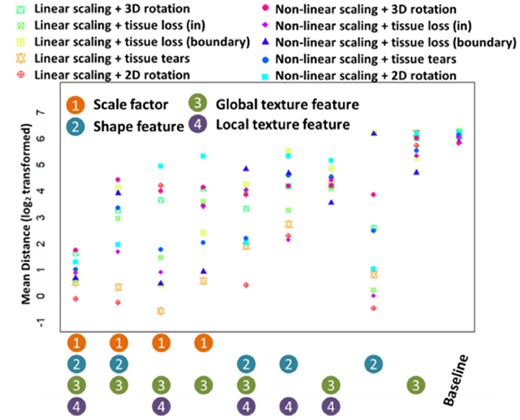
Matching performance on the simulated data. Matching performance of 10 methods (baseline method, the proposed ARMBIS method and eight partial ARMBIS without some of the grouped features, including scaling factor, global texture, shape feature or local texture features) under 10 different simulation settings. The matching accuracy is measured by the mean distance between the matched index of the image and the ground truth

Open in new tab Download slide

Correction for rotation angles estimated by the shape feature leads to better matching performance. The model without scaling factor estimation can be taken as a special case of ARMBIS for single image matching. However, such image matching highly depends on the shape features and is accurate only when the shape features have strong discriminative ability under the scenarios of linear and non-linear scaling with 2D rotations (the matching distances range from 1.68 to 4.00). Supplementary Table S2 summarizes the performance of different types of features in the simulated studies.

3.2 Real applications

The performance of ARMBIS is tested on MRI, DAPI and GFP images.

MRI images: We used 13 MRI image sets to test the performance of our propose matching method. The MRI experiments were performed by the BrukerBiospec 70/20USR small animal MR system (BrukerBioSpin MRI, Ettlingen, Germany) operating at 300 MHz (7.0 T). The experiment process is described in detail in Supplementary Methods 1.4. These MRI images went through BET (Brain Extraction Tool) (Smith, 2002) for extraction of mouse brains. BET removes non-brain tissue (e.g. brain skull) from an image of the whole head. It uses a deformable model that evolves to fit the brain's surface with the aid from a set of locally adaptive model forces. After BET, some manual refinement was performed to remove some obvious errors so as to derive clean and accurate mouse brain regions.

DAPI and GFP images: We randomly chose nine DAPI and nine GFP images to test the performance of the proposed ARMBIS. The coronal brain sections with red or green fluorescence signal came from C57 mice with anterograde or retrograde transsynaptic virus tracers (Beier et al., 2011; Smith et al., 2000). PRV531 (3.7 × 10⁹ PFU/ml) and VSV-mCherry (5.0 × 10⁷genomix copies/ml) were provided by Brain VTA (BrainVTA Co., Ltd., Wuhan, China). PRV531 or VSV-mCherry was injected into the unilateral olfactory bulb in C57 mice. After three days, the mice were euthanized by cardiac perfusion, and the brain was removed and post-fixed for further histological studies. Then 40 μm coronal frozen slices were acquired. The upper whole steps were detailed described in our previous study (Zhang et al., 2017). For VSV tracing samples, one out of six consecutive slices was stained with DAPI. Selection of PRV tracing samples was similar with VSV group, but they were not treated by DAPI. The fluorescent images of brain slices were obtained from Olympus VS120 microscope (Olympus, Japan).

3.2.1 Performance of curve fitting

In well-ordered MRI image sequences, the images on both ends of each sequence are much smaller than those in the middle, suggesting a single peak in the extracted geometric feature sequence which should be considered in pattern matching. Curve fitting is used to estimate a scaling factor between a query image sequence and a reference image sequence. The curve fitting results for the MRI query image sets are shown in Supplementary Figures S7–S19. Due to large variations and intrinsic noises in imaging, feature curves, especially feature curves of query images have low resolution and are not smooth. This makes it difficult to represent these curves by piecewise line segments. However, the proposed curve smoothing and matching approach is robust to such noises, and scaling factors estimated by the four geometric features are very consistent with a mean absolute difference of 8%.

3.2.2 Discriminative power of the proposed features

In our proposed method, the texture and contour shape features can provide an additional verification to each other when one category of the features does not have much discriminative ability for some image deformations. In Figure 3A, the seventh query image has some distinct texture features and thus its similarities to the reference images have an anticipated major peak located at #124. But the shape similarity curve has several points with similar similarities around the best matched index, leading to ambiguous estimations. Figure 3B shows an example query image whose shape features are more informative than its texture features. In both (A) and (B), the discriminative power of the unscaled texture feature is much lower than the scaled global texture feature.

Fig. 3.

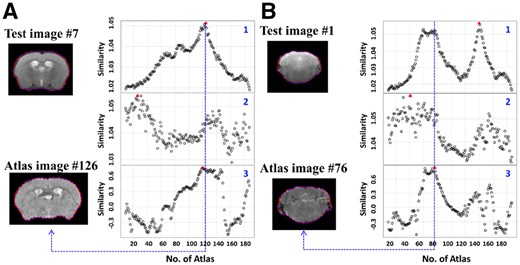
Examples of texture and shape feature curves. (A) (1) The scaled global texture similarities, (2) The unscaled global texture similarities, (3). The shape similarities between the seventh image (up) in the query sequence and all the images in the atlas image set 1. The red triangle indicates the location of the maximum on each curve. Atlas #126 (bottom) is the best matched image in the atlas image set. (B) (1) The scaled global texture similarities, (2) The unscaled global texture similarities, (3) The shape similarities between the first image (up) in the query sequence and all the images in the atlas image set 1. Atlas #76 (bottom) is the best matched image in the atlas image set

Open in new tab Download slide

3.2.3 Image sequence matching accuracy

The most important criterion for evaluating image matching is matching accuracy. Figure 4 shows examples of matching a query image sequence 1 to three brain atlas image sets. The images at the beginning and the end of the query image sequence do not have distinct texture characteristics while the query images #5, #6, #7, #8 and #9 have rich texture features. All these matching results are consistent with the best matched indices provided by the experts. It is worth noting that the final best matched image indices are given by the aforementioned decision scheme for multiple atlases. Similar to the simulation study, we compare the performance of the full and partial ARMBIS models as well as the baseline method using the MRI dataset 1. As shown in Supplementary Figure S20, the integration of all the features gives rise to robust results in the real situation. More results from the MRI image sequences are shown in Supplementary Figures S21–S33.

Fig. 4.

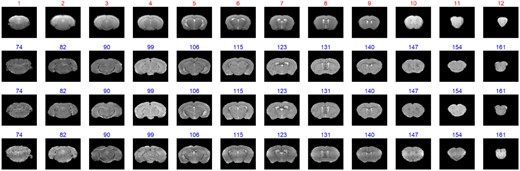
The matching result of the MRI images. The red numbers are the indices of the test image, and the blue numbers are the indices of the best matched indices from atlas image sequence (The whole matching results for the 10 atlas image sets are shown in Supplementary Fig. S21)

Open in new tab Download slide

3.2.4 Single image matching accuracy

Figure 5 shows the results for a single DAPI image and a single GFP image. The fluorescent images with detailed structures and textures have much higher resolution than the MRI images. Some regions of the fluorescent images have extremely high intensity due to fluorescence staining and this may be a challenge for comparison based on global features. The regional texture features can be taken as an additional verification of the final matching results. In this example, not all the orders of the image patches $V_{D^{j (p)}}^{m_{tj}'}$ are summed up in Equation (9). For an image $j$ ⁠, we select $(P - 2)$ patches with the smallest $V_{D^{j (p)}}^{m_{tj}'}$ instead of all the patches to avoid the influence of non-informative patches due to large individual variations in the patches compared to the atlas images. More results of single DAPI and GFP image matching results are shown in Supplementary Figures S34–S51. All of the matching results are consistent with the best matched images provided by the experts.

Fig. 5.

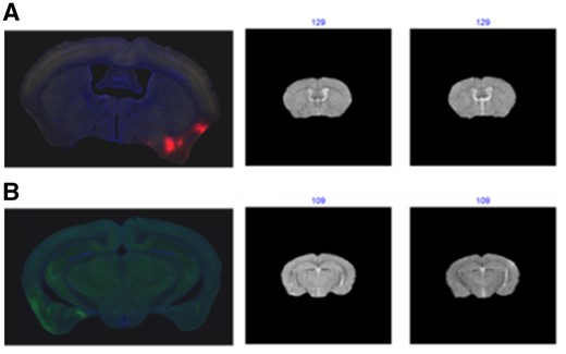
(A) The matching results of DAPI images. (B) The matching result of the GFP. The blue numbers are the indices of the best matched indices from 2 atlas image series (The whole matching results for the 10 atlas image sets are shown in Supplementary Figs S34 and S43)

Open in new tab Download slide

4 Discussion

In this study, we develop a novel algorithm, ARMBIS, for matching brain image sequences to established atlas image sequences. Image sequence matching here can be considered as a classification task in which each class has only one training sample but training samples are spatially related. Unlike traditional intensity-based image matching approaches, ARMBIS utilizes both texture features of image contents and shape features of image contours. The two types of features are complementary to each other and are mechanistically integrated to make a final decision. Applications of ARMBIS to the simulated and real data show outstanding performance. The main contributions of this study are summarized as follows: (i) ARMBIS can be applied to multiple types of brain images if query images are properly processed into gray-scale images. (ii) ARMBIS takes advantage of continuity in the geometric feature space from 3D brain images to overcome the problem of different scales in query image and atlas sequences. If an image sequence is not incomplete, ARMBIS provides an alternative solution based on a hierarchical decision approach using both global and local features of the original images. (iii) ARMBIS utilizes a piecewise linear approximation for the representation of functional imaging data. Images are represented as feature curves which are further partitioned into segments by detecting important sign change points as break points. An optimization function is implemented to identify the best matched region and an optimal scaling factor for a query image sequence and an atlas one. (iv) ARMBIS can handle large variations in query images and reference atlas images that may lead to evenly spaced best matched atlas images through a dynamic programming-based procedure with the constraints on the order and maximal distance.

After several best matched candidate images are determined by the global features, regional features are used for precise image matching to eliminate the effect of image defections or individual structure variations. The similarities between the patches of a query image and those of the atlas images can be taken as additional verification of the matching results given by the global features. In Equation (9), if all the patches are considered, $S_{t}$ may be affected by the patches which have large variations compared with the atlas image, and the matching results are more likely to be same as the results from the global features. However, if only a few most informative patches are considered, the model is more robust to noises. As shown in Supplementary Figure S3, the orders of the most similar atlas images for the patches #1 and #2 are much larger than the other patches and this may be caused by image defections or individual variations at the upper left region of the image. Therefore, if we discard these two patches in the calculation by Equation (9), $\sum_{p = 1}^{P - 2} V_{D^{j (p)}}^{m_{tj}'}$ will be 10, leading to the best matched index of 126, a more accurate matching. In general, selecting the optimal number of patches highly depends on image quality. In all our experiments, $P$ is chosen as 6 and 4 patches are used in the sum of the orders.

In the simulation study, we perform 3D rotations by rotating the original image along its Z-axis and then find the most similar image in the atlas space. The results show that our model can handle well such image deformations. In real data, sometimes slicing direction or interslice distance between query images is too different from that in an atlas to find any matched images. Such cases can be determined by a pre-defined similarity threshold and will be matched against new atlases that can be generated through 3D reconstruction based on the original atlas until the overall similarities are acceptable. Matching brain image sequences to reference atlases is the very first step to understand the function of the brain. Here we do not consider the problem of image registration. Another limitation with the current study is that only different types of coronal brain slices are tested. The future work will be focused on (i) evaluating ARMBIS by horizontal or sagittal images, extending ARMBIS to different mouse atlases, and integrating ARMBIS and 3D brain image registration.

Funding

This work was supported, in part, a Seed Fund from the Icahn School of Medicine at Mount Sinai (to B.Z.), a grant from the National Institutes of Health [U01AG046170] (to B.Z.) and a grant from the Youth Innovation Promotion Association of Chinese Academy of Sciences [Y6Y0021004] (to J.W.).

Conflict of Interest: none declared.

References

Agarwal

et al. (

2016

) Robust registration of mouse brain slices with severe histological artifacts. In: Proceedings of the Tenth Indian Conference on Computer Vision, Graphics and Image Processing, ACM, Indian Institute of Technology, Guwahati.

Agarwal

et al. (

2017

) Geometry processing of conventionally produced mouse brain slice images. arXiv preprint arXiv: 1712.09684.

Bai

et al. (

2012

)

Atlas-based automatic mouse brain image segmentation revisited: model complexity vs. image registration

Magn. Reson. Imaging

789

–

798

Beier

K.T.

et al. (

2011

)

Anterograde or retrograde transsynaptic labeling of CNS neurons with vesicular stomatitis virus vectors

Proc. Natl. Acad. Sci. USA

108

15414

–

15419

Google Scholar

Crossref

WorldCat

Cleveland

W.S.

Devlin

S.J.

(

1988

)

Locally weighted regression: an approach to regression analysis by local fitting

J. Am. Statist. Assoc

596

–

610

Google Scholar

Crossref

WorldCat

Cootes

T.F.

et al. (

1993

) The use of active shape models for locating structures in medical images. In Biennial International Conference on Information Processing in Medical Imaging, Springer, Berlin, Heidelberg.

Cootes

T.F.

et al. (

1995

)

Active shape models-their training and application

Comput. Vis. Image Understand

–

Google Scholar

Crossref

WorldCat

Jain

et al. (

2005

)

Score normalization in multimodal biometric systems

Pattern Recogn

2270

–

2285

Google Scholar

Crossref

WorldCat

Lowe

D.G.

(

2004

)

Distinctive image features from scale-invariant keypoints

Int. J. Comp. Vis

–

110

Google Scholar

Crossref

WorldCat

et al. (

2005

)

A three-dimensional digital atlas database of the adult C57BL/6J mouse brain by magnetic resonance microscopy

Neuroscience

135

1203

–

1215

Midroit

et al. (

2018

)

Non-imaged based method for matching brains in a common anatomical space for cellular imagery

J. Neurosci. Methods

304

136

–

145

Milborrow

Nicolls

(

2008

)

Locating facial features with an extended active shape model

. In:

European Conference on Computer Vision

. pp.

504

–

513

Berlin, Heidelberg

Mulloy

P.G.

(

1994

)

Smoothing data with faster moving averages

Stocks Commod

–

Google Scholar

OpenURL Placeholder Text

WorldCat

L.L.

et al. (

2012

)

Large-scale neuroinformatics for in situ hybridization data in the mouse brain

Intl. Rev. Neurobiol

104

159

–

182

Google Scholar

Crossref

WorldCat

Ojala

et al. (

2002

)

Multiresolution gray-scale and rotation invariant texture classification with local binary patterns

IEEE Trans. Pattern Anal. Mach. Intell

971

–

987

Google Scholar

Crossref

WorldCat

Poo

M-m.

et al. (

2016

)

China brain project: basic neuroscience, brain diseases, and brain-inspired computing

Neuron

591

–

596

Smith

B.N.

et al. (

2000

)

Pseudorabies virus expressing enhanced green fluorescent protein: a tool for in vitro electrophysiological analysis of transsynaptically labeled neurons in identified central nervous system circuits

Proc. Natl. Acad. Sci. USA

9264

–

9269

Google Scholar

Crossref

WorldCat

Smith

S.M.

(

2002

)

Fast robust automated brain extraction

Hum. Brain Mapp

143

–

155

Swain

M.J.

Ballard

D.H.

(

1991

)

Color indexing

Int. J. Comput. Vis

–

Google Scholar

Crossref

WorldCat

Toga

A.W.

(

2015

) Brain Mapping: An Encyclopedic Reference. Academic Press, San Diego, 2015. ISBN 978- 0-12-397316-0. URL http://www.sciencedirect.com/science/referenceworks/9780123973160.

Vincent

Soille

(

1991

)

Watersheds in digital spaces: an efficient algorithm based on immersion simulations

IEEE Trans. Pattern Anal. Mach. Intell

583

–

598

Google Scholar

OpenURL Placeholder Text

WorldCat

Wold

et al. (

1987

)

Principal component analysis

Chemom. Intell. Lab. Syst

–

Google Scholar

Crossref

WorldCat

et al. (

2009

) Bundling features for large scale partial-duplicate web image search. In: IEEE Conference on Computer Vision and Pattern Recognition, 2009. IEEE, Miami, Florida.

Yushkevich

P.A.

et al. (

2006

) 3D mouse brain reconstruction from histology using a coarse-to-fine approach. In:

International Workshop on Biomedical Image Registration

. Springer, Berlin, Heidelberg.

Zhang

et al. (

2017

)

Whole-brain mapping of the inputs and outputs of the medial part of the olfactory tubercle

Front. Neural Circuits

This article is published and distributed under the terms of the Oxford University Press, Standard Journals Publication Model (https://dbpia.nl.go.kr/journals/pages/open_access/funder_policies/chorus/standard_publication_model)

Associate Editor:

Download all slides

Month:	Total Views:
May 2019	20
June 2019	8
July 2019	2
August 2019	10
September 2019	17
October 2019	8
November 2019	11
December 2019	8
January 2020	30
February 2020	10
March 2020	12
April 2020	5
May 2020	4
June 2020	10
July 2020	6
August 2020	5
September 2020	3
October 2020	10
November 2020	14
December 2020	9
January 2021	4
February 2021	7
March 2021	4
April 2021	20
May 2021	18
June 2021	11
July 2021	23
August 2021	11
September 2021	15
October 2021	21
November 2021	16
December 2021	11
January 2022	7
February 2022	11
March 2022	22
April 2022	23
May 2022	15
June 2022	14
July 2022	31
August 2022	30
September 2022	102
October 2022	127
November 2022	43
December 2022	88
January 2023	42
February 2023	18
March 2023	18
April 2023	85
May 2023	29
June 2023	24
July 2023	17
August 2023	35
September 2023	26
October 2023	25
November 2023	32
December 2023	34
January 2024	31
February 2024	32
March 2024	27
April 2024	30
May 2024	34
June 2024	37
July 2024	23
August 2024	9
September 2024	10
October 2024	7
November 2024	15
December 2024	26
January 2025	4
February 2025	9
March 2025	21
April 2025	15
May 2025	5

Article Contents

ARMBIS: accurate and robust matching of brain image sequences from multiple modal imaging techniques

Abstract

1 Introduction

2 Methods

2.1 Feature extraction

2.1.1 Extraction of scale and rotation invariant shape features

2.1.2 Scaling factor estimation by robust curve fitting of the feature series

2.1.3 Extraction of texture features

2.2 Image matching

2.3 Robust matching for single query image

3 Results

3.1 Simulation studies

3.2 Real applications

3.2.1 Performance of curve fitting

3.2.2 Discriminative power of the proposed features

3.2.3 Image sequence matching accuracy

3.2.4 Single image matching accuracy

4 Discussion

Funding

References

Supplementary data

Citations

Views

Altmetric

Email alerts

Citing articles via

Latest

Most Read

Most Cited

Looking for your next opportunity?

Article Contents

ARMBIS: accurate and robust matching of brain image sequences from multiple modal imaging techniques Free

Abstract

1 Introduction

2 Methods

2.1 Feature extraction

2.1.1 Extraction of scale and rotation invariant shape features

2.1.2 Scaling factor estimation by robust curve fitting of the feature series

2.1.3 Extraction of texture features

2.2 Image matching

2.3 Robust matching for single query image

3 Results

3.1 Simulation studies

3.2 Real applications

3.2.1 Performance of curve fitting

3.2.2 Discriminative power of the proposed features

3.2.3 Image sequence matching accuracy

3.2.4 Single image matching accuracy

4 Discussion

Funding

References

Supplementary data

Citations

Views

Altmetric

Email alerts

Citing articles via

Latest

Most Read

Most Cited

Looking for your next opportunity?

This Feature Is Available To Subscribers Only

ARMBIS: accurate and robust matching of brain image sequences from multiple modal imaging techniques