Graphlet Laplacians for topology-function and topology-disease relationships

Abstract

1 Introduction

Systems biology is flooded with large scale ‘omics’ data. Genomic, proteomic, interactomic, metabolomic and other data, are typically modelled as networks (also called graphs). This abundance of networked data started the fields of network biology, allowing us to uncover molecular mechanisms of a broad range of diseases, such as rare Mendelian disorders (Smedley et al., 2014), cancer (Leiserson et al., 2015) and metabolic diseases (Baumgartner et al., 2018). In personalized medicine, network analysis is applied to the tasks of biomarker discovery (Li et al., 2015), patient stratification (Gligorijević et al., 2016) and drug repurposing (Durán et al., 2018).

Many network analysis methods use the Laplacian matrix as it captures the global wiring patterns of a network (see Section 1.1). These methods include spectral clustering, spectral embedding and network diffusion. Each of these families of methods relies on the fact that the eigendecomposition of the Laplacian matrix naturally uncovers network clusters (see Section 1.2). Applications of spectral embedding include visualizing genetic ancestry (Lee et al., 2010) and pseudo-temporal ordering of single-cell RNA-seq profiles (Campbell et al., 2015). Applications of spectral clustering include detection of functional sub-network modules in single-cell genomic networks (Bartlett et al., 2017) and identification of functional modules in co-regulatory networks (Luo et al., 2018). Network diffusion methods are widely used for protein function prediction (Cao et al., 2013) and discovery of disease genes and disease modules, see Cowen et al. (2017) for a full review.

1.1 Laplacian matrix definition

The Laplacian, $L$⁠, is defined as $L=D−A.$ The symmetrically normalized Laplacian, L^sym, is defined as $Lsym=D−1/2LD−1/2$⁠.

1.2 Laplacian matrix eigendecomposition

1.3 Matrix alternatives to the Laplacian

Vicus is an alternative to the Laplacian that captures the intricacies of a network’s local structure (Wang et al., 2017) based on network label diffusion. Label diffusion is defined as P = BQ, where the n × d matrix Q assigns the n nodes of network G to one of d possible labels (for labelled nodes), B is an n × n diffusion matrix, and the reconstructed matrix P is an n × d matrix used for predicting labels for unlabelled nodes. To give Vicus its ‘local’ interpretation, the label diffusion process determining B is constrained to diffuse information of each node only to its direct neighbourhood. Under given assumptions and defining Vicus as $LV=(I−BT)(I−B)$⁠, it was shown that Q can be learned as the eigenvectors of $LV$⁠. As Q captures the local connectivity between nodes that is implied by the ‘localized’ diffusion matrix B and can be computed as the eigenvectors of $LV$⁠, Vicus is interpreted as a Laplacian matrix. Vicus is applied to protein module discovery and ranking of genes for cancer subtyping (Wang et al., 2017).

1.4 Problem

All Laplacian-based applications are based on the same underlying principle of guilt by association, inferring information on a given node based on the group of nodes it is most tightly connected with. However, alternative approaches have inferred information on a given node based on the shape of its interaction pattern, typically independent of the identity of the nodes it is interacting with. These alternative approaches are based on graphlets, small connected sub-graphs (see Section 2.1 for a formal definition), to capture the local topology around a node in a network. For example, graphlet-based methods have been applied to predict protein function (Davis et al., 2015; Milenković and Pržulj, 2008) and to identify new cancer genes (Milenković et al., 2010) directly from the similarities in terms of their interaction patterns in PPI networks.

Alternatives to the Laplacian matrix that take local topology into account have been suggested. The k-path Laplacian captures the influence of long-range interactions between nodes, but ignores short-range interactions. Vicus captures local topology around each node as the strength of its connection to its neighbours after applying a localized label diffusion algorithm. Although Vicus is focused on capturing local topology, it lacks interpretability from a structural perspective.

1.5 Contribution

We introduce the Graphlet Laplacian, allowing us to analyse nodes based on their network neighbourhoods, whilst restricting the pattern of their interactions to that of a pre-specified graphlet. Hence, each graphlet (Fig. 1A) has its own corresponding Graphlet Laplacian. We generalize spectral embedding, spectral clustering and network diffusion to utilize Graphlet Laplacians. Through graphlet-generalized spectral clustering of model networks and biological networks, we show that different Graphlet Laplacians capture different local topologies. By applying graphlet-generalized spectral embedding, we visually demonstrate that Graphlet Laplacians capture biological functions as well. We quantify this through graphlet-generalized spectral clustering analysis. We show that Graphlet Laplacians are not only as biologically relevant as alternative Laplacian matrices, but also capture complementary biological functions. Finally, by graphlet-generalized diffusing of pan-cancer gene mutation scores on the human PPI network, we show that Graphlet Laplacians capture complementary disease mechanisms. We compare our results against those based on alternative state the art Laplacian matrices. A similar methodology based on network motifs was presented by Benson et al. (2016) for spectral clustering of directed networks.

Fig. 1.

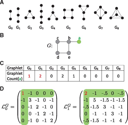
Illustration graphlets and Graphlet Laplacians. Node a is coloured in green throughout. The graphlet counts of node a for graphlet G₀ and G₁ are coloured in red throughout. (A) All graphlets with up to 4 nodes, labelled G₀ to G₈. (B) A dummy network. (C) A vector of graphlet counts describing the local topology of node a in the example network, G. Node a touches graphlet G₀ via edge (a, b). Node a touches graphlet G₁ twice, via paths a-b-c and a-b-e. (D) The Graphlet Laplacians for graphlets G₀ and G₁, applied on the network, G, shown in B. The diagonal elements correspond to the graphlet counts of each node; e.g. $L0G(1,1)$ is equal to 1, the number of times node a touches graphlet G₀, $L1G(1,1)$ is equal to 2, the number of times node a touches graphlet G₁. The off-diagonal elements correspond to the number of times two nodes touch a given graphlet together, scaled by $size(Gk)−1$⁠. $L0G(1,2)=−1$⁠, as a and b form G₀ once and $size(G0)−1=1$⁠. $L1G(1,2)=−1$⁠, as a and b form G₁ twice and $size(G1)−1=2$

Open in new tabDownload slide

2 Materials and methods

2.1 Graphlet Laplacian definition

We generalize the Laplacian matrix so that it can capture the local topology of a network around a node in a broader sense than the identity of its direct neighbours. One of the most sensitive methodologies to capture network topology around a node are graphlets: small, connected, non-isomorphic, induced sub-graphs of a large network (Pržulj et al., 2004). All graphlets up to four nodes are depicted in Figure 1A. To illustrate how graphlets can be used to quantify the local topology around a node, consider node a in the dummy network presented in Figure 1B. Graphlet G₁ (i.e. a three node path) that touches node a can be found in this dummy network twice: via paths a-b-c and a-b-e. Node a is said to touch G₁ twice. By making these counts for a given node over all graphlets, the local network topology for a given node can be quantified by means of a vector, as illustrated for node a in Figure 1C. Here, we see that node a can be found as part of an edge once (G₀), as part of a three node path twice (G₁), never as part of a triangle (G₂) and so on.

Having established that by counting how often a node touches graphlets can be used to quantify its local topology, we go on and generalize the concept of the Laplacian to that of a Graphlet Laplacian by generalizing the definitions of adjacency and degree to ones based on graphlets. First, we define two nodes u and v of G to be graphlet-adjacent with respect to a given graphlet, G_k, if they simultaneously touch G_k. Going back to our previous example, we find that nodes a and b are graphlet-adjacent w.r.t. graphlet G₁ twice, as G₁ can be induced on the dummy network twice: via paths a-b-c and a-b-e, each time including both nodes a and b. Similarly, nodes a and c and nodes a and e are graphlet-adjacent only once, w.r.t. graphlet G₁.

2.2 Graphlet Laplacian properties

To allow for an easy interpretation of the Graphlet Laplacian for each graphlet, G_k, we introduce the two-step transformation function, T, which maps graph G to its Graphlet Laplacian representation: $T(G,Gk)=LkG$⁠. First, T converts $G={V,E}$ to a weighted network $G′={V,E′}$⁠, where the weight of each edge (u, v) in $G′$ corresponds to $auvk/(size(Gk)−1)$ measured in G. Next, T converts $G′$ to its standard Laplacian representation. This shows that the Graphlet Laplacian can be interpreted as the Laplacian of an undirected weighted network. Therefore, the Graphlet Laplacian retains the following key properties of the Laplacian:

• The Graphlet Laplacian, $LkG$⁠, is symmetric and positive semi-definite.

• The smallest eigenvalue is 0 and the corresponding eigenvector is the constant vector $1$⁠. eigenvector

• The Graphlet Laplacian has n non-negative, real-valued eigenvalues: $0=λ1k≤λ2k,…,λnk$⁠.

• The multiplicity of the eigenvalue 0 equals the number of connected components in $G′$⁠, which we refer to as graphlet-based components.

2.3 Spectral embedding

2.4 Spectral clustering

Spectral clustering uncovers groups of nodes in a network that form densely connected network clusters. By generalizing spectral clustering to Graphlet Laplacian-based spectral clustering, we are able to identify network components that are densely connected with respect to a given graphlet. Many different variations of spectral clustering exist (Von Luxburg, 2007). Aiming for a balanced clustering, we generalize normalized spectral clustering as defined by Ng et al. (2002) to use different Laplacians including Graphlet Laplacians, all denoted by a generic $L$ in algorithm 1. We skip the normalization step (i.e. step 1) for Vicus, as Vicus is already normalized.

For each network, we determine the numbers of clusters, d, by using the rule of thumb: $d≈n/2$ (Kodinariya and Makwana, 2013). In the Supplementary Section S1, we present the justification for this approach, based on inspection of the spectra of different Laplacian matrices of each network. Because of the heuristic nature of spectral clustering, we perform 20 runs for each clustering and consolidate them into a single clustering applying ensemble clustering (Ghosh and Strehl, 2002).

2.5 Network diffusion

2.6 Topological dissimilarity of networks

2.6.1 Graphlet correlation distance

The Graphlet Correlation Distance (GCD-11) is the current state of the art heuristic for measuring the topological distance between networks (Yaveroǧlu et al., 2014). First, the global wiring pattern of a network is captured in its Graphlet Correlation Matrix (GCM), an 11 × 11 symmetric matrix comprising the pairwise Spearman’s correlations between 11 different graphlet-based counts over all nodes in the network. The GCD between two networks is computed as the Euclidean distance of the upper triangle values of their GCMs.

2.6.2 Non-graphlet based network descriptors

The difference between the following non-graphlet based network descriptors can be used to measure the distance between two networks:

• The degree distribution is the distribution of node degrees over all nodes. It is summarized as a vector of counts, i.e. the kth value is the number of nodes that have degree k. To measure the distance between two networks, this vector is first rescaled to reduce the contribution of higher degree nodes. The pairwise distance between two networks is the Euclidean distance between their rescaled degree distribution vectors. For more details, see (Yaveroǧlu et al., 2014).

• The diameter of a connected network is the maximum shortest path distance that is observed among all node pairs. The distance between two networks is the absolute difference of their diameters.

• The average clustering coefficient is the total number of three node cliques in the network over the number of possible three node cliques in the network. The distance between two networks is the absolute difference of their average clustering coefficient.

2.7 Cluster enrichment analysis

2.8 Data

2.8.1 Real biological network data collection

We create three types of molecular interaction networks for human and baker’s yeast (Saccharomyces cerevisiae) by collecting the following data: experimentally validated protein–protein interactions (PPIs) from IID version 2018-05 (Kotlyar et al., 2016) and BioGRID version 3.4.161 (Stark et al., 2006), genetic interactions from the same version of BioGRID and gene co-expressions from COXPRESdb version 6.0 (Okamura et al., 2015).

2.8.2 Random model network generation

For each of the following 8 random network models, we generate 10 networks containing 2000 nodes at edge density of 1.5%: Erdős–Rényi random graphs (ER) (Erdős Paul and Rényi Alfréd, 1959), generalized random graphs with the degree distribution matching to the input graph (ER-DD) (Newman, 2010), Barabási–Albert scale-free networks (SF) (Barabási and Albert, 1999), geometric random graphs (GEO) (Penrose, 2003), geometric graphs that model gene duplications and mutations (GEO-GD) (Pržulj et al., 2010), stickiness-index based networks (Sticky) (Pržulj and Higham, 2006), popularity–similarity optimization graphs (PSO) (Papadopoulos et al., 2012) and non-uniform PSO graphs (nPSO) (Muscoloni and Cannistraci, 2018). A summary on the basic properties of these networks and how to generate them can be found in Supplementary Section S2.1.

2.8.3 Biological annotations

For each gene in our biological networks, we collect the most specific experimentally validated biological process annotations (BP), cellular component annotations (CC) and molecular function annotations (MF) present in the Gene Ontology (GO) (Ashburner et al., 2000).

2.8.4 Cancer gene annotations

We collect the pan-cancer gene mutation frequency scores computed by Leiserson et al. (2015) for the purpose of detecting pan-cancer disease modules. Leiserson et al. (2015) collected raw pan-cancer mutation data, such as SNV’s, indels and CNA’s, from the TCGA database (Kandoth et al., 2013). These data were filtered to exclude statistical outliers and include only the samples (corresponding to a patient) for which SNV and CNA data were available. The resulting dataset contains mutations on 11 565 genes across 3110 patients in cancers across 20 different tissues. Additionally, we collect the sets of known cancer driver genes in all available tissues from IntOGen (Gonzalez-Perez et al., 2013) and Cosmic (Futreal et al., 2004).

3 Results and discussion

We investigate the potential usage of Graphlet Laplacians to analyse network data via embedding, clustering and network diffusion experiments. We consider Graphlet Laplacians for graphlets with up to four nodes. We compare our results to the state of the art Laplacian matrices: the standard Laplacian, the k-path Laplacian and Vicus. We consider path lengths up to three for the k-path Laplacian, corresponding to the maximum size of the considered graphlets underlying the Graphlet Laplacian. We set Vicus’ diffusion parameter to 0.9, as this value is recommended in the original paper (Wang et al., 2017) and leads to the largest number of enriched functions (see Section 3.2).

3.1 Graphlet Laplacians capture different local topologies

While the standard Laplacian simply captures the direct neighbourhoods of nodes and can be used to cluster densely connected nodes together, the graphlet-based neighbourhood captured by our Graphlet Laplacian allows for clustering of nodes that strongly participate in a given graphlet of interest. Because different graphlets capture different local topologies around nodes in a network (e.g. G₃ involve paths while G₈ involves cliques), clusters obtained by using different Graphlet Laplacian are expected to possess different topological features, which we assess as follows.

To assess if two graphlet Laplacians, $LiG$ and $LjG$⁠, capture different topologies, we apply each Laplacian to cluster nodes in a network using Graphlet Laplacian-based spectral clustering. The resulting clusters are used to partition the network into two sets of sub-networks, by inducing the sub-networks from each clustering. $LiG$ and $LjG$ capture different topologies if the corresponding sets of sub-networks have significantly different topology, which we measure by the overlap of two distributions: the distribution of GCD-11 distances between the sub-networks produced from $LiG$ with the sub-networks produced from $LjG$ and distribution of GCD-11 distances between the sub-networks produced from $LiG$⁠. The two Graphlet Laplacians capture statistically significantly different topologies if the Wilcoxon–Mann–Whitney U-test (MWU) between the two distributions of distances is lower than or equal to 5% (see Fig. 2 for the case of $L0G$ and $L4G$⁠). For each type of model network, we perform this test ten times and report the least significant P-value for each pairwise comparison of Graphlet Laplacian-based sub-networks. We also considered the following non-graphlet based network distance measures: degree distribution distance, diameter distance and average clustering coefficient distance (see Section 2.6.2). In general and independent of the network distance measure used, clusters obtained from different Graphlet Laplacians are typically statistically significantly topologically different at the 5% significance level. This is true across all of our biological networks and most of our model networks, with some exceptions in geometric models which are known to have homogeneous structure. Thus, Graphlet Laplacians not only capture network cluster that have different topology, but can also be used to measure the structural homogeneity of a given network.

Fig. 2.

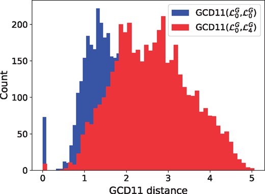
Comparison of topological distance distributions between sub-networks captured by two different Graphlet Laplacians in the human PPI network. The distribution of GCD-11 distances between the sub-networks from $L0G$ (in blue) is statistically significantly different from the distribution of GCD-11 distances between the sub-networks from $L0G$ and the sub-networks from $L4G$ (in red) with MWU P-values ≤5%. This means that$L0G$ and $L4G$ capture different topologies in the human PPI network

Open in new tabDownload slide

We illustrate this by investigating how the parameters of the PSO/nPSO model networks influence the topological homogeneity of the networks generated, see Supplementary Figures S7–S9. At a low temperature (i.e. nodes are connected to nearby nodes) and low number of communities (i.e. the angle of each node is sampled from a univariate Gaussian), both types of networks are homogeneous. As temperature increases, newly added nodes are more uniformly connected in space (i.e. are more randomly connected), making the generated PSO and nPSO networks closer to ER networks, thus breaking the homogeneous structure. In nPSO networks, increasing the number of communities increases the homogeneity of the networks. This effect is stronger at lower temperatures.

3.2 Different Graphlet Laplacians capture different biological functions

In biological networks, genes having similar functions tend to be densely connected to each other (Hartwell et al., 1999), which is why spectral clustering based on the standard Laplacian matrix has been used to uncover functional regions in networks (Bu et al., 2003). Alternatively, graphlets have been used to show that functionally related genes tend to be similarly wired, independent of them being densely connected (Milenković and Pržulj, 2008). As graphlet Laplacians capture both types of information, they should also capture biological functions.

To informally visualize this, we perform spectral embedding. We focus on the embedding of the yeast GI network, for which we use 14 core biological process annotations defined by Costanzo et al. (2016). We illustrate the spectral embedding of the symmetrically normalized $L3G$ Graphlet Laplacian in Figure 3. The embeddings of the other Laplacian matrices of the yeast GI network can be found in the Supplementary Section S3. As seen in Figure 3, the spectral embedding of $L3G$ correctly groups and separates the biological processes of ‘nuclear cytoplasmic transport’, ‘metabolism/mitochondria’, ‘Golgi/endosome/vacuole sorting’ and ‘Chrom. seg./kinetoch./spindle/micro tub.’. In the Supplementary Material, we illustrate that Vicus and the Laplacian fail to find any grouping at all, placing all of the nodes in the same dense cluster. Embeddings based on $L2P$ and $L3P$ succeed in separating different genes into different clusters, but without grouping them in a biologically meaningful way.

Fig. 3.

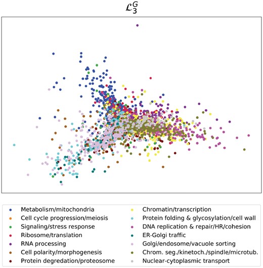
Capturing biological functions with Graphlet Laplacian $L3G$⁠. 2D spectral embedding of the yeast GI network using the Graphlet Laplacian for G₃. Points represent genes and are colour-coded with 14 core biological process annotations defined by Costanzo et al. (2016)

Open in new tabDownload slide

Next, we aim to quantify this result by measuring the difference in functions captured by different Graphlet Laplacians. We apply Graphlet Laplacian-based spectral clustering for each graphlet on our set of human molecular networks and assess the functional enrichments in terms of the percentage of clusters enriched and the total number of annotations enriched (Fig. 4). Additionally, we create a baseline to validate the statistical significance of our enrichment results. We perform the same experiment 100 times with randomized GO-annotations. We do this by swapping the sets of gene annotations in the molecular networks such that no gene has its original set of annotations.

Fig. 4.

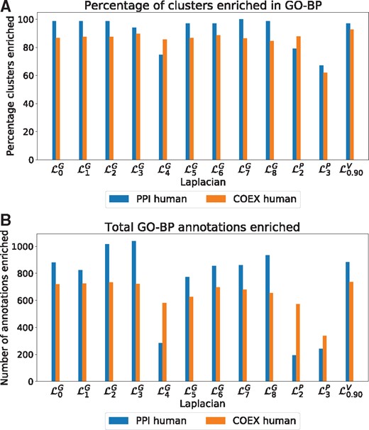
Cluster quality. (A) For our set of human molecular networks (colour-coded), the percentage of clusters enriched in BP annotations, with clusters obtained based on spectral clustering using different Laplacian matrices (x-axis). (B) For our set of human molecular networks, the total number of enriched GO-BP annotations in clusters obtained based on spectral clustering using different Laplacian matrices (x-axis)

Open in new tabDownload slide

First, we observe that clusterings based on all Graphlet Laplacians but $L4G$ tend to be of similar quality as those based on the standard Laplacian or Vicus, both in terms of percentage of clusters enriched as well as total number of annotations enriched. $L2P and L3P$ capture the lowest amount of functions in PPI networks, both in terms of percentage of clusters enriched and GO-BP annotations enriched. Secondly, in our randomized experiment with randomized GO-annotations, we consistently find 0% of the clusters to be enriched, regardless of the type of Laplacian matrix used. This shows that all Laplacian-based enrichments are statistically significant. We find similar results in yeast, see Supplementary Section S5. In the Supplementary Material, we additionally observe that for each network and annotation type, there is always at least one Graphlet Laplacian that shows a larger number of the total number of enriched annotations than Vicus. We conclude that Graphlet Laplacians are at least as biologically relevant as the standard Laplacian, k-path Laplacian and Vicus.

Having established that Graphlet Laplacian-based clusters capture biological functions, we quantify the overlap in their enriched functions. In the Supplementary Section S6, we calculate the Jaccard Index between the sets of enriched functions corresponding to each Graphlet Laplacian. For GO-BP enrichments in clusterings on the human PPI and COEX networks, the average Jaccard Index is 0.22 and 0.30, respectively, meaning that different Graphlet Laplacians capture different functions. To further demonstrate this point, we present the number of GO-BP functions that are enriched only in the clustering obtained by a particular Graphlet Laplacian in Figure 5. We observe that each type of Laplacian matrix shows a tendency to capture some distinct biological functions, indicating the link between the biological function and the topology of these diverse molecular networks. The same is observed for GO-MF and GO-CC annotations, both in yeast and human networks (see the Supplementary Section S7). Combining this observation with our previous results, we can conclude that Graphlet Laplacian-based spectral clustering allows for distinguishing different sets of similarly wired network components that are not only biologically relevant, but may also capture complementary biological functions.

Fig. 5.

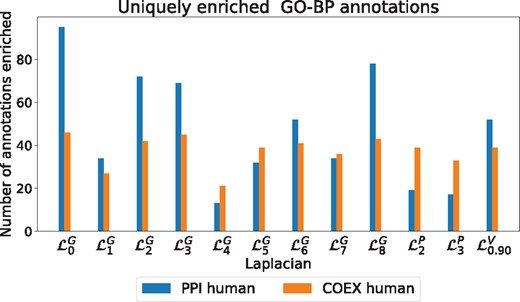
GO-BP uniquely enriched. The number of annotations that are uniquely enriched in clusterings based on the indicated Laplacian matrix for each biological network (colour coded)

Open in new tabDownload slide

3.3 Different Graphlet Laplacians capture complementary sets of pan-cancer-related genes

Laplacian-based approaches towards predicting cancer-related genes are based on guilt by association: genes which tend to be connected to frequently mutated genes are used as cancer gene predictions. Here, we show that by considering the different shapes (i.e. graphlets) by which genes can be connected to frequently somatically mutated genes, complementary cancer mechanisms can be captured.

We do this by diffusing (see Section 2.5) the gene mutation frequency scores (see Section 2.8.4) on the human PPI network based on different Graphlet Laplacian matrices. Network diffusion is a method underlying many of the different approaches of cancer gene prioritization (Cowen et al., 2017). We prioritize genes as potential cancer-related genes according the highest diffused score first. We measure the quality of these scores using the area under the precision-recall (PR) curve and the area under the receiver operator characteristic (ROC) curve. We assume a gene is correctly classified as a cancer-related gene if it is known to be a cancer driver gene in at least one type of cancer (see Section 2.8.4). We observe that accuracy is independent of the Graphlet Laplacian used and on par with the standard Laplacian, with an average area under the PR and ROC curves of 0.21 and 0.78 respectively. In terms of accuracy Graphlet Laplacian-based scores consistently outperform those based on k-path or Vicus, which achieve an average area under the PR and ROC curve of 0.17 and 0.74 and 0.14 and 0.73 respectively (see Supplementary Figs S17 and S18).

In Figure 6, we evaluate the overlap between the top hundred highest ranking cancer-related genes per Laplacian, measured using the Jaccard Index. We observe five distinct clusters of different Laplacian matrices capturing different sets of cancer-related genes. Importantly, diffusion based on three sets of Graphlet Laplacians (⁠$L{2,5,7}G$⁠, $L{1,3,4,6}G$ and $L{8}G$⁠) provide scores dissimilar to those achieved using the standard Laplacian (the average Jaccard Index of each cluster with the standard Laplacian-based scores being 0.79, 0.87, 0.65 respectively). Conversely, the highest scoring genes based on $L{2,3}P$ prove to overlap greatly with those based on the standard Laplacian (the average Jaccard Index being 0.91). Vicus-based diffusion provides cancer-related gene scores dissimilar from all other Laplacian matrices, be it at lower accuracy, as shown above. Similar results are obtained applying graphlet-generalized diffusion on the human COEX network, as shown in Supplementary Sections S8 and S9. We conclude that Graphlet Laplacian-based diffusion can be used to find complementary sets of cancer-related genes.

Fig. 6.

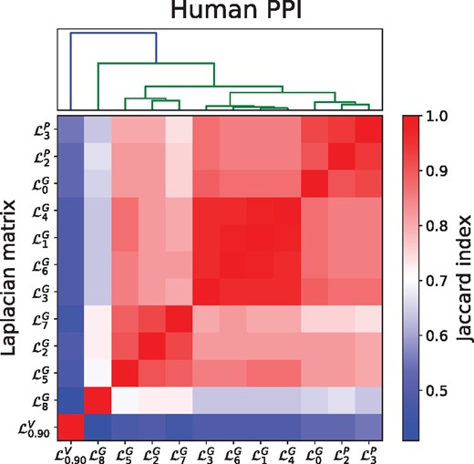
Overlap of highest scoring cancer-related genes. Evaluating the overlap in the sets of the top 100 highest scoring genes based on different Laplacians measured by the Jaccard Index, with scores computed by performing network diffusion of mutation frequency scores on the human PPI network

Open in new tabDownload slide

4 Conclusion

In this article, we introduce Graphlet Laplacians for simple networks to simultaneously capture graphlet-based topological information and neighbourhood membership information. We demonstrate that they can straightforwardly be plugged into current Laplacian-based network analysis methods widely used in systems biology, using spectral clustering, spectral embedding and network diffusion as example applications.

Through our generalized spectral embedding and spectral clustering methods on real and model networks, we show that different Graphlet Laplacians capture sub-networks having distinct local topologies and that are enriched in different, but complementary sets of biological annotations. Finally, we show that our generalized network diffusion of pan-cancer gene mutation scores resulted in complementary sets of cancer-related genes for gene prioritization dependent on the underlying graphlet. In all the tested applications, our Graphlet Laplacians perform as good as and often better than k-path and Vicus Laplacians, while being directly interpretable.

As indicated, Graphlet Laplacians can directly replace the traditional Laplacian matrix in state-of-the-art network analysis methods, allowing them to consider alternative ways of how nodes are connected. For instance, our Graphlet Laplacians could be used to extend embedding methods such as hyper-coalescent embedding (Muscoloni et al., 2017), which may result in more relevant community detections in biological networks and in more accurate analyses of the dynamics of cells’ biological processes. Furthermore, Laplacian matrices are used in data-integration frameworks to incorporate prior knowledge (e.g. via so-called graph regularizations in matrix factorization-based data integration). Thus, using our Graphlet Laplacians in such data-integration frameworks could result in biologically more accurate patient stratifications, biomarker discoveries and drug-target interaction predictions (Gligorijević et al., 2016).

Finally, the applications of Graphlet Laplacians are not limited to biology, as the generalized network-analysis tools are applicable in any discipline that uses network representations, including physics, social sciences and economy.

Funding

This work was supported by the European Research Council (ERC) Starting Independent Researcher [Grant 278212]; the European Research Council (ERC) Consolidator [Grant 770827]; the Serbian Ministry of Education and Science [Project III44006]; the Slovenian Research Agency [project J1-8155]; the Prostate Project and UCL Computer Science departmental funds.

Conflict of Interest: none declared.

References