


Abstract
The information criterion of minimum message length (MML) provides a powerful statistical framework for inductive reasoning from observed data. We apply MML to the problem of protein sequence comparison using finite state models with Dirichlet distributions. The resulting framework allows us to supersede the ad hoc cost functions commonly used in the field, by systematically addressing the problem of arbitrariness in alignment parameters, and the disconnect between substitution scores and gap costs. Furthermore, our framework enables the generation of marginal probability landscapes over all possible alignment hypotheses, with potential to facilitate the users to simultaneously rationalize and assess competing alignment relationships between protein sequences, beyond simply reporting a single (best) alignment. We demonstrate the performance of our program on benchmarks containing distantly related protein sequences.
The open-source program supporting this work is available from: http://lcb.infotech.monash.edu.au/seqmmligner.
Supplementary data are available at Bioinformatics online.
1 Introduction
Identifying the evolutionarily retained similarities between macro-molecular sequences remains an indispensable first step of many biological studies (Lesk, 2017). Comparison of sequences are carried out using the computational technique of alignment. An alignment is used as a surrogate for how two (or more) sequences are evolutionarily related and provides a quantitative measure of their similarity (Allison et al., 1992, 1999; Barton and Sternberg, 1987; Lesk, 2017).
Alignment techniques commonly depend on choosing a model for relating two sequences with stated parameters to score matched and penalize unmatched (gap) regions in any alignment. However, in practice, it is left for the users to fine-tune these parameters in their quest for meaningful sequence relationships. This parameter tuning remains a ‘black art based on trial and error’ (Do et al., 2005), and several studies have underscored major problems with parameter tuning and demonstrated the conflicting effects this has on resulting alignments (Do et al., 2006; Löytynoja and Goldman, 2008; Rivas and Eddy, 2015; Vingron and Waterman, 1994). These limitations were best summarized by Löytynoja and Goldman (2008) in their observation that ‘alignment is still a highly error-prone step in comparative sequence analysis’.
The problem becomes more pronounced when comparing amino acid sequences of proteins, which additionally rely on substitution matrices. A protein sequence alignment gives a one-to-one correspondence between amino acids symbols, and substitution scores are used to quantify these correspondences. A substitution matrix over the standard amino acid alphabet is parameterized on a distance (or alternatively a similarity) parameter between sequences, and conveys the mutability of one amino acid changing into another. PAM (Dayhoff et al., 1978) and BLOSUM (Henikoff and Henikoff, 1992) are widely used series of substitution matrices.
Yet, in the use of these substitution matrices, there remains a severe disconnect between the substitution scores (used to score the matched amino acid correspondences) and gap parameters (used to penalize the unmatched regions of alignments). Previous studies have shown that, different protein sequence alignment programs with varying choices of substitution and gap parameters convey radically different alignments (Barton and Sternberg, 1987; Blake and Cohen, 2001; Fitch and Smith, 1983; Löytynoja and Goldman, 2008; Vingron and Waterman, 1994). Further, the confidence of reported relationship in an alignment plummets when comparing protein sequences from the twilight zone [by common consensus defined as sequences sharing less than 35% sequence identity (Doolittle, 1986)]. Do et al. (2006) observed that the correctness of a reported sequence alignment is highly questionable when it is below a 25% sequence identity.
Beyond the problem with tuning alignment parameters, another major shortcoming is that most current programs report a single alignment. Many studies have demonstrated that optimizing an objective function under a specified model of sequence relatedness does not necessarily imply an optimization in homology (Fitch and Smith, 1983; Durbin et al., 1998; Levy Karin et al., 2019; Redelings and Suchard, 2005; Rosenberg, 2009) (see Supplementary notes for a more detailed discussion).
Aforementioned deficiencies provide a motivation for the work presented here. Specifically for comparing protein sequences, we attempt to rectify: (i) the problem of arbitrariness of alignment parameters, (ii) the disconnect between substitution scores and gap parameters, and (iii) the lack of a rigorous statistical framework where all competing alignments can be simultaneously rationalized and assessed, beyond reporting just a single (best) alignment.
Our work uses the statistical inductive inference method of minimum message length (MML) encoding (Allison, 2018; Wallace, 2005; Wallace and Boulton, 1968) to compare the relatedness of protein sequences in information-theoretic terms, measurable in bits. In this framework, any alignment between protein sequences is a string generated by a three-state alignment machine with match, insert and delete states. This allows us to compute robust probability estimates of sequence alignments.
Independently, we infer from a set of 118 384 structural alignments between protein domains, the parameters of Dirichlet probability distributions that allow us to link the distance parameter of existing substitution matrices (e.g. parameter ‘n’ of PAM-n) with the state machine (transition probability) parameters that produce the three-state alignment strings. These parameters provide a substantial statistical rationalization of the otherwise ad hoc use of gap penalties. In statistical learning theory, the Dirichlet distribution is often used as a prior distribution over the parameters of finite-state models. It is a conjugate prior for multistate models, which implies that the resultant posterior is also a Dirichlet distribution (Allison, 2018).
Furthermore, building on these inferred Dirichlet priors, we design a statistical compression based alignment methodology with automatically estimated parameters, to compute the marginal probability landscape of any given protein sequence pair (e.g. see Fig. 1(a)). Marginal probability estimation (Trumpler and Weaver, 1953) applied to sequence alignment provides a powerful technique to highlight the relationship between sequences, by marginalizing over all the alignments between the sequences. Specifically, for a pair of sequences , any cell (i, j) in this landscape gives the product of marginal probabilities that the prefixes and suffixes are related. This involves integrating over all possible alignments passing through the cell (i, j) in any of the three alignment states. Since these are rigorous estimates of probabilities of relationship between sequences, the resultant landscape allows the user to visualize not just the most probable alignment, but also interactively query closely competing alignments passing through any cell (e.g. see Fig. 1(b)).
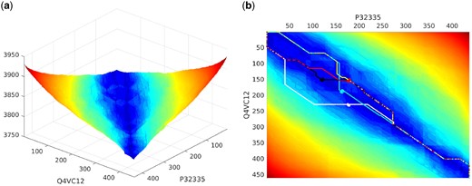
(a) Marginal probability landscape to visualize the relatedness of two protein sequences over all competing alignments. (b) Most probable alignments passing through a set of specific cells (i, j) in the sequence landscape, including the most probable over all cells (shown in black)
Most importantly, the MML framework provides a natural statistical significance test when assessing any alignment or comparing one with another. This is measurable in bits of compression with respect to the null model message length that gives the Shannon’s information content (Shannon, 1948) [related to the Kolmogorov complexity (Kolmogorov, 1963)] of each of the two sequences independently summed up.
Finally, asymptotic computational complexity to compare sequences under this framework and generate these marginal alignment landscapes is . Any specific competing alignment can be probed and reported in time after the initial effort.
We note that our work develops and significantly extends the basic ideas of finite state models for alignment introduced by Allison et al. (1992, 1999), Powell et al. (2004) and Sumanaweera et al. (2018). More generally, other noteworthy attempts at probabilistic modeling of alignments, although with different aims and motivations, include: Durbin et al. (1998), Zhu et al. (1998), Do et al. (2005, 2006) and Rivas and Eddy (2015). See supplementary Section S4 for an overview of the literature on this topic.
2 Materials and methods
2.1 Primer on MML criterion
MML encoding is a Bayesian method for hypothesis (model) selection that is grounded in information and coding theory (Allison, 2018; Wallace, 2005; Wallace and Boulton, 1968).
For any hypothesis H on observed data D, their joint probability is given by: . Independently, Shannon (1948) in his Mathematical Theory of Communication quantified the information content (measurable in bits) in any event E that occurs with a probability of Pr(E) as . In other words, I(E) is the shortest message length required to communicate losslessly the information conveyed by E. Applying Shannon’s insight, the joint probability between any hypothesis and data can be expressed in terms of Shannon’s information content as: . This can be rationalized as the length of the message communicated between an imaginary transmitter-receiver pair; the transmitter’s goal is to encode and send the data D over a chosen hypothesis H as efficiently as possible, so that the receiver can decode the message and losslessly recover D. The transmission message is in two parts: the first deals with encoding and sending the hypothesis, taking I(H) bits; the second deals with encoding the data given the hypothesis, taking bits.
More importantly, implicit in this framework is a null hypothesis (or model). The null model message involves stating D without venturing a hypothesis—i.e. stating D raw, but as efficiently as possible—taking INULL (D) bits. If the best hypothesis H*, the one that yields the shortest message length over the space of all possible hypotheses, does not beat the null model (i.e. ), then that hypothesis has to be rejected.
The MML paradigm for hypothesis selection provides a direct tradeoff between hypothesis complexity I(H) and its fit to the data : a more complex hypothesis results in a higher value of I(H) but may describe the data better with a lower value of , and vice versa. Furthermore, MML ensures complete transparency in communication. Any information that is not common knowledge or based on preconceived notions implicit in the data has to be included as part of the message sent by the transmitter. Otherwise the transmission is not lossless, and the message sent will be indecipherable by the receiver. No parameters can be hidden from the communication, and the precision of statement of real-valued parameters has to be directly dealt with as part of the MML framework (Wallace, 2005; Wallace and Freeman, 1987). Note, the practical realization of MML is built on strong statistical foundations developed over 40 years in the general statistical learning literature outside molecular biology (Allison, 2018; Wallace, 2005; Wallace and Freeman, 1987).
2.2 Protein sequence comparison in MML paradigm
Any alignment hypothesis over the sequences specifies a string over three states, match (m), insert (i) and delete (d), generated from a three-state machine with unknown parameters (Fig. 2). For a given pair of sequences, these state-machine parameters are to be inferred in concert with the distance parameter (also unknown) between the two sequences. (These details together with computation of the message length terms denoted in Equation 1 are specified in Sections 2.3–2.4.)
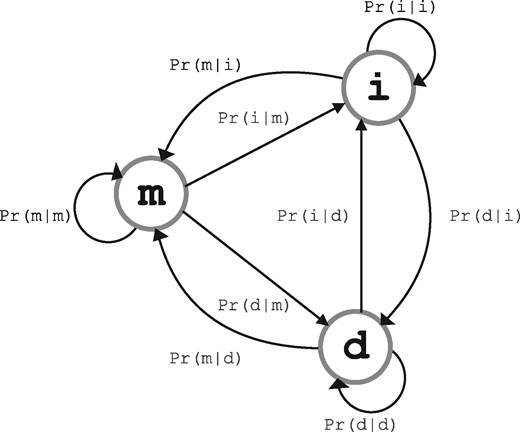
Three-state machine for alignment string modeling
The summation over all possible alignments as per Equation 2 gives the marginal probability of the relationship between two sequences . The corresponding message length takes bits. Marginal probability provides a general and unbiased probability estimate of the relationship compared with that of any specified alignment (see Equation 1). It follows that .
In general, if , the hypothesis that are related is accepted. Specifically, if , then provides the best hypothesis of their relationship. Otherwise, both the marginal and optimal hypotheses are rejected.
2.3 MML inference of Dirichlet priors on state machine parameters as a function of sequence distance
As introduced in Section 2.2, any alignment of is a string produced by a three-state machine. Figure 2 illustrates the three-state machine over match (m), insert (i) and delete (d) states, with nine one-step transition probabilities. This machine has an implicit constraint that the sum of one-step transitions out of each state should add up to the probability of 1: . Consistent to the accepted practice of aligning macromolecular sequences, the following transition symmetries are additionally enforced in this work: ; ; ; . With these symmetries, the three-state alignment machine now has three free (unknown) parameters. Notionally, these are: (i) , (ii) and (iii) . Once these free parameters are estimated, the enforced symmetries allow the remaining transition probabilities to be assigned as follows: ; ; ; .
Therefore, our use of the symmetric three-state alignment machine entails estimation of the three free parameters distributed over a 1-simplex for , and a 2-simplex for and . We note that the unit -simplex involves L1 normalized, k dimensional vectors (Allison, 2018). Thus, a vector of k probabilities corresponding to mutually exclusive events can be represented as a point in a unit (k − 1)-simplex.
To estimate the state machine parameters, especially as a function of the distance between two sequences, we undertake the following one-time probabilistic modeling exercise using Dirichlet distributions over simplexes. These derived Dirichlet priors support the parameter estimation in our MML based protein sequence comparison framework.
2.3.1 Preparation of datasets for inference
We randomly sampled from SCOP (ver. 2.07) (Murzin et al., 1995) a set of 118 384 protein structural domain-pairs, containing 47 687 domain-pairs that are related at a family level and 70 697 domain pairs related more distantly at a superfamily level. See Supplementary Section S3 for details of the domain-pairs and the method used for random selection. All 118 384 domain pairs are structurally aligned using their 3D coordinate information (Collier et al., 2017). These structural alignments are used in our modeling exercise below.
Furthermore, these structural alignments are partitioned into subsets based on the observed sequence-distance between their corresponding SCOP domain-pairs. A surrogate measure of sequence-distance was provided by Dayhoff et al. (1978) in terms of Point Accepted Mutation (PAM) units. They derived PAM-1 transition probability matrix over the standard 20-letter amino acid alphabet that gives the probability of one amino acid mutating into another in a unit PAM distance step. The PAM-1 matrix can be generalized to any PAM-n via exponentiation, PAM-n = (PAM-1)n, which gives the probability of one amino acid mutating into another in n PAM distance steps. (Indeed other notions of sequence-distances could be used (e.g. BLOSUM). We use PAM in this work only for its convenience that allows us to generalize it systematically to arbitrary distances between sequences.)
Therefore, for each structural alignment in our set of alignments, we identify the best integer n in the range [1, 1000] that maximizes the probability of matched amino acids in that alignment using PAM-n, yielding 1000 subsets of alignments. These alignment subsets are used to infer 1000 Dirichlet priors, one for each subset of observed alignments as a function of their corresponding sequence-distance.
Dirichlet distributions are conjugate priors for multistate models over finite-state strings with any fixed k discrete states. Multistate models define k parameters (of which k − 1 are free) that lie in a (k − 1)-simplex. In our work, for each subset corresponding to the sequence-distance parameter n in the range [1, 1000], we have a set of observed three-state alignment strings. Our goal is to model these and infer Dirichlet prior parameters over the corresponding multistate transition probability parameters. As discussed above, the three free parameters of the symmetric three-state alignment machine (see Fig. 2) can be decomposed and modeled using Dirichlet distributions over a unit 1-simplex (accounting for the free parameter ), and a unit 2-simplex (accounting for the remaining free parameters and ).
Below we summarize the MML method of inferring free parameters from an observed dataset containing finite-state strings, along with their optimal Dirichlet prior parameters.
2.3.2 Estimation of finite state transition probabilities over any Dirichlet prior
2.3.3 Estimation of Dirichlet parameters over finite-state strings
and deal with the message length terms required to transmit the Dirichlet and state parameters, respectively. Finally, deals with the transmission of all finite-state strings in A, using the corresponding state parameters and Dirichlet prior (see Supplementary Section S2).
The Dirichlet parameter estimator defined by Equation 5 is used on the subsets of structural alignments defined over PAM-based sequence distances in the range , to derive 1000 Dirichlet priors as a function of sequence-distance parameter n (see Section 3). These precomputed priors are employed to assign alignment state machine parameters when comparing any two sequences, as discussed below.
2.4 Practical considerations for protein sequence comparison and alignment using the MML framework
2.4.1 Estimation of null-model message length
Equation 3 in Section 2.2 involves the computation of null model message lengths of individual amino acid sequences, S and T. This in turn involves the statement of each amino acid symbol in these sequences using their respective null probabilities.
The MML estimate of the null probability for any amino acid symbol is computed over the large corpus of protein sequences derived from the Universal Protein Resource (UniProt-Consortium et al., 2017). Specifically, corresponding to the 20-state amino acid strings are computed using Equation 4 by setting the 20-dimensional Dirichlet parameter vector to . This is same as using a uniform prior for the estimation of the null probabilities. We note that the estimation of null probabilities for amino acid sequences is one-off and independent of any particular sequence comparison.
Applying the above equation to S and T yields the required null-model message length, .
2.4.2 Estimation of alignment-model message length
Equation 1 in Section 2.2 gives the length of the two-part message to communicate any sequence pair over an alignment hypothesis . The first part encoding deals with the statement of an alignment hypothesis as a three-state string over the finite state machine with m, i and d states, as depicted in Figure 2. From the Dirichlet modeling exercise carried out in Section 2.3, for any stated PAM-n distance between with , we have an associated Dirichlet prior. In this work, we chose the mode (i.e. point of maximum probability density) of the nominated Dirichlet distribution to define the nine state transition parameters. Since Dirichlet priors can be treated as common knowledge between the transmitter and receiver, the transmitter needs only to state the parameter n. (Under a uniform assumption of , the code length to state n is estimated as bits.) Once n is decoded, the receiver gains knowledge of the precise state transition probabilities used in the transmission of .
The second part encoding involves explaining the amino acid symbols in using the alignment hypothesis and the distance parameter n (both communicated in the first part). Each position in the alignment indicates one of the three possibilities: (i) an amino acid symbol is unmatched (delete); (ii) an amino acid symbol is unmatched (insert); and (iii) a pair of amino acid symbols and are matched (match).
This joint probability estimate is a symmetric measure independent of the assumed order of the two sequences being considered. Negative logarithm of this joint probability gives the Shannon’s information content (i.e. statement length) of communicating the matched amino acid pair. The total length of stating over any alignment , , sums up the statement lengths over all matched and unmatched positions in , as described above.
2.4.3 Dynamic programming algorithm to compute the marginal probability of sequences
Thus, the negative logarithm of the marginal probability that are related is given by , plus the constants associated with stating n, taking bits, and the sum of lengths of the two sequences, . Furthermore, in the above set of DPA recurrences, replacing –LSE function by min function yields the method to compute the best alignment hypothesis under our MML framework.
Finally, an approach similar to the bisection method is used to identify the corresponding optimal distance parameter n that yields the best estimate for , and separately for , searching over the domain . In each iteration, this approach truncates the search domain from [lo, hi] to either or by removing either the first or the last quarter of the domain after evaluating the marginal probability (or similarly, the best alignment hypothesis) at those two quarter points. The value of lo upon termination is taken to be the optimal estimate of n.
2.4.4 Marginal probability landscapes
In order to generate the marginal probability landscapes that allow users to visualize all competing alignments simultaneously, the following approach is used. For a given , the DPA is run in the forward direction (i.e. natural direction of the sequences). This yields the inferred distance parameter n and the dynamic programming history matrices and . Using the inferred distance parameter from the forward run, the DPA is run in the backward direction (i.e. reverse direction of the sequences), yielding the history matrices and .
A combined landscape matrix is derived by computing, for each cell (i, j), the negative LSE function over the following nine arguments: (i) , (ii) , (iii) , (iv) , (v) , (vi) , (vii) , (viii) and (ix) .
Any cell (i, j) in this landscape gives the product of marginal probabilities that the prefixes and suffixes are related. The marginal probability landscape provides insightful visualization of alignment relationships between two sequences. It also allows users to interactively generate competing alignments passing through any specified cell (i, j) in the landscape (see Section 3).
3 Results and discussion
3.1 Inferred Dirichlet priors
Using the inference method described in Section 2.3, we derived 1000 Dirichlet priors to model the observed distributions of state machine parameters, as a function of sequence distance measured in terms of Point Accepted Mutations (Dayhoff et al., 1978) (see Supplementary Section S3).
Figure 3(a) shows all the 1000 distributions of the free parameter associated with the match state. This parameter influences the observed lengths of the matched blocks produced by the three-state machine. These lengths are geometrically distributed, and the probability of seeing a matched block of length L is . The expected length of the matched block is given by . Furthermore, due to the enforced symmetry of state transitions from match state to insert or delete states (see Section 2.3), we have: . This value informs the probability of observing a gap in any alignment produced by the state machine. Figure 3(c) plots the expected probability of observing a gap as a function of distance n, when is set to the mean (red) and mode (blue) values under the Dirichlet distributions shown in Figure 3(a). We notice the trend that the probability of a gap increases linearly with n in the range [1, 350], and stays relatively flat when n > 350. This linear trend agrees with the observations by Gonnet et al. (1992) and Benner et al. (1993).
![Visualization of the inferred Dirichlet distributions modeling the three free parameters of the finite-state machine, and their associated statistics. (a) One-simplex distributions of Pr(m|m) associated with the match, as a function of sequence-distance n∈[1,1000]. (b) 2-simplex distributions of Pr(i|i) and Pr(m|i) associated with insert (and by symmetry, delete), as a function of sequence-distance n∈{1,40,80,120,160,200,400,600,800}. Since the values of Pr(i|i) (estimated from the mode) are in the range of [0.81, 0.93] for n∈[1,1000], its simplex support shown above has been truncated for clarity to the range of [0.5, 1.0]. (c) The distribution of mean and mode values of Pr(i|m)+Pr(d|m) under the Dirichlet priors, as a function of n. (d) The distribution of expected gap lengths derived from the mode-estimate of Pr(i|i) under the inferred Dirichlet priors](https://oup.silverchair-cdn.com/oup/backfile/Content_public/Journal/bioinformatics/35/14/10.1093_bioinformatics_btz368/3/m_bioinformatics_35_14_i360_f3.jpeg?Expires=1750072653&Signature=CA8HinHHE2GS7nF45IhNaQzyXqGirmmSMmEEQYzTvqADneJPXgB~yIu-6TWeX9pz-ORM3vxhho3SEMCNQmhiysBxMBD4tHeBpUEDCMzi0HdsaCNTL4sPJ7UfVwOj0eKkuziog53kdDGrs1Sr6OQgTqHhCVi7k2p48ypbc5oknD-Prqy0dOsh6tjVQPSVJeijv07j~GEhv8FDbHKr-dCElGAsMA3uPlXT560Z7K0gKo2Jn8A8QF8Ia0OyV7eWEuQ69kd-4hQrVpoar9N9wCEmHqv0REWmAWWJOeb~tc158DlM26Tt6RAqcWwKdNMc-lGd3nHghr1uwp3-BUU~GVjvOA__&Key-Pair-Id=APKAIE5G5CRDK6RD3PGA)
Visualization of the inferred Dirichlet distributions modeling the three free parameters of the finite-state machine, and their associated statistics. (a) One-simplex distributions of associated with the match, as a function of sequence-distance . (b) 2-simplex distributions of and associated with insert (and by symmetry, delete), as a function of sequence-distance . Since the values of (estimated from the mode) are in the range of [0.81, 0.93] for , its simplex support shown above has been truncated for clarity to the range of [0.5, 1.0]. (c) The distribution of mean and mode values of under the Dirichlet priors, as a function of n. (d) The distribution of expected gap lengths derived from the mode-estimate of under the inferred Dirichlet priors
On the other hand, Figure 3(b) shows a small selection of nine Dirichlet distributions, for specific values of , associated with the insert state parameters. (By symmetry, insert and delete state parameters are equivalent.) The heat map shows the inferred concentration (refer Section 2.3.2) of the probability density about the mode shown as a yellow dot (at the center of the heat map). The black dot shows the mean under the same distribution. The three corners (bottom-left, bottom-right, top) of each triangle (denoting the 2-simplex support for L1-normalized transition probabilities of insert state) show the points where , and become exactly 1, while remaining two parameters become 0.
As n increases, it can be seen from Figure 3(b) that also increases (see mean and mode—yellow and black dots in the plots—approach the bottom-left corner). This parameter influences the observed length of an insert (and, by symmetry, delete) block in an alignment. Again, these block lengths are geometrically distributed, with the probability of seeing a gap of length L defined by , and whose expected gap length is given by .
Figure 3(d) plots the expected gap length as a function of n with the mode estimate assigned to the parameter . On average, the expected gap length is about five amino acid residues for n in the range [1, 120], and barring a few outliers at n = [43, 44, 45, 91, 94], the trend is flat. Examining the source structural alignment data of these outliers (i.e. n-based alignment subsets on which the Dirichlet priors have been inferred), we find protein domain pairs with circularly permuted amino acid sequences and other pairs with plastic deformations in their structures. We note that a circular permutation between proteins results in a non-sequential relationship. Enforcing a sequence alignment on such a relationship yields regions that cannot be sequentially-aligned, which are then misinterpreted as long gaps. Similarly, domain pairs with plastic deformations have the same effect on gap lengths.
Further, in the range of , we see in Figure 3(d) that the expected gap length increases linearly as a function of n. This contradicts the observation by Benner et al. (1993) who have stated that ‘the distribution of gap size is essentially independent of the evolutionary distance between two sequences, with only a modest decrease in average gap length at increasing PAM distance’.
Finally, in the range of n > 350, the expected gap length in Figure 3(d) shows a noisy-yet-flat trend line, averaging about 13 to 15 amino acid residues. This trend more likely reveals the limits of applicability of PAM (Markov) matrix, and its convergence to its stationary distribution for large n (Dayhoff et al., 1978). To test this, we measure the Kullback–Leibler (KL) divergence of each amino acid with varying PAM-n against its stationary distribution. We note that the KL-divergence between any two discrete probability distributions f and g over N mutually exclusive events, measures the additional number of bits required to encode samples drawn from f using g (i.e. it measures their relative Shannon entropy): By varying the value of , we computed the KL-divergence between each amino-acid’s substitution probability distribution (i.e. each column of PAM-n) and the stationary distribution (i.e. the eigenvector associated with the dominant eigenvalue of 1 of PAM matrices). Figure 4 plots the KL-divergence for each amino acid with varying PAM-n. We observe that, for n > 350, most columns of PAM-n (i.e. amino acid substitution probabilities) converge to the stationary distribution. This indicates the limits of PAM’s ability to differentiate amino acid substitutions at larger evolutionary distances.
![Kullback–Leibler divergence between each amino acid related column in the PAM-n matrix and its stationary distribution, measured in bits. The black partitions define the [1, 120], [120, 350] and [350, 1000] regions corresponding to the PAM-n ranges where we see different trends for the expected gap length](https://oup.silverchair-cdn.com/oup/backfile/Content_public/Journal/bioinformatics/35/14/10.1093_bioinformatics_btz368/3/m_bioinformatics_35_14_i360_f4.jpeg?Expires=1750072653&Signature=hhIey4tRaFiFFKRe6WbYG4yGkxEiy8LaGiTdpTAUc3zlN5hcIDamF2-WyhIUZ2Ax6oHDRaPm-SrWh5a7qGUdwRUIE8bntN7XNY5PtQJqaD4uU1Kpoauq91170cm6Sh3V9xSN5SaNVECPVzCbYnQ9SvrIz7Bl85GCm14dHzHKlUPuV5ekwfE2ad75lmwZFGH6tsQuYMxk8knWQ51Pkkdbl1QFTD3RUQgmZZyj9fYca2JpJKEiZGMadoxufIeLPsSKCLpv~lktTvqceoz~PDZQJEnrXzac3HyTConKfEplUQinKBAFXyBJxKUWr8T0mo3dYGu0VLaEAXx7OW6hnFqmiQ__&Key-Pair-Id=APKAIE5G5CRDK6RD3PGA)
Kullback–Leibler divergence between each amino acid related column in the PAM-n matrix and its stationary distribution, measured in bits. The black partitions define the [1, 120], [120, 350] and [350, 1000] regions corresponding to the PAM-n ranges where we see different trends for the expected gap length
3.2 Comparison with other programs on distantly related pairs of protein sequences
We used two types of benchmark datasets to test the performance of our sequence comparison framework. The first is a set of experimentally verified remote orthologs reported by Szklarczyk et al. (2012), containing a total of 877 protein sequence pairs spread over two groups. The second is the entire twilight zone dataset from SABmark (Van Walle et al., 2005) containing 10 250 protein sequence pairs, spread over 209 groups.
Specifically, the dataset of Szklarczyk et al. (2012) include, in the first group, 405 pairs of human orthologous fungal mitochondrial proteins found in Saccharomyces cerevisiae, and in the second group, 472 pairs of orthologs found in Schizosaccharomyces pombe. Their average percentage sequence identity is reported as 27.7%, with about 40% of this dataset having pairs with <25% sequence identity and 36% between 25% and 35% sequence identity.
We ran our MML based alignment program in two separate modes. The first mode finds the best alignment hypothesis that minimizes the message length term given in Equation 1. This yields the statistic, together with the information measures of alignment complexity and alignment fidelity . The second mode, which is the main focus of this work, is the one that estimates the negative logarithm of the marginal probability as per Equation 2 that yields statistic. Both and are compared with their corresponding null model message length, as per Equation 3, yielding the bits of ‘Compression’ statistic.
Further, we compare the results of this dataset against seven widely-used protein sequence alignment programs: ClustalW (Larkin, 2007), CONTRAlign (Do et al., 2006), KAlign (Lassmann and Sonnhammer, 2005), MAFFT (Katoh and Standley, 2013), MUSCLE (Edgar, 2004), ProbCons (Do et al., 2005) and T-COFFEE (Notredame et al., 2000). We evaluate the performance across all these program using the ‘Compression’ statistic. For each alignment produced by the programs, we infer the best parameters that minimize their measure. This allows us to compare various message length terms against to find its ‘Compression’. We consider as hits (i.e. pairs that are correctly identified as related), only those alignments whose is shorter than (refer statistical significance test in Section 2.2). This allows us to compute the percentage of the total number of sequence pairs that pass the null hypothesis test for significance (%-Hits). Table 1 presents these results across the two benchmark groups of human remote orthologs (Szklarczyk et al., 2012). In the table, we report the corresponding median values (across the whole group) against , and ‘Compression’ entries.
Comparison of various programs over two benchmark datasets: Human versus fungal ortholog groups reported by Szklarczyk et al. (2012), and SABmark (Van Walle et al., 2005) twilight zone dataset
| Human remote orthologs of fungal mitochondrial proteins | SABmark proteins | ||||||||
|---|---|---|---|---|---|---|---|---|---|
| Human versus S.cerevisiae (405 pairs) | Human versus S.pombe (472 pairs) | Twilight (10 250 pairs) | |||||||
| Program | %-Hits | Compression | %-Hits | Compression | %-Hits | ||||
| ClustalW | 71.85 | 117.4 | 2678.1 | 82.6 | 74.58 | 110.3 | 2575.0 | 77.1 | 1.7951 |
| CONTRAlign | 71.11 | 117.8 | 2679.9 | 75.7 | 72.03 | 108.8 | 2573.6 | 70.7 | 2.3512 |
| KAlign | 73.83 | 134.3 | 2639.3 | 84.9 | 74.79 | 24.8 | 2533.1 | 81.8 | 2.4878 |
| MAFFT | 70.79 | 163.9 | 2622.1 | 81.8 | 71.91 | 150.9 | 2535.7 | 76.7 | 1.8187 |
| MUSCLE | 73.83 | 136.5 | 2639.3 | 86.1 | 76.06 | 129.8 | 2539.1 | 84.9 | 2.4976 |
| ProbCons | 70.12 | 143.5 | 2639.3 | 78.9 | 71.61 | 130.4 | 2543.9 | 75.9 | 1.6683 |
| TCoffee | 69.14 | 141.8 | 2640.9 | 76.5 | 71.19 | 130.8 | 2544.4 | 71.1 | 1.6390 |
| MML () | 79.26 | 119.1 | 2666.5 | 93.7 | 80.51 | 109.5 | 2548.85 | 94.2 | 4.1399 |
| MML () | 94.57 | N/A | N/A | 125.0 | 94.49 | N/A | N/A | 117.9 | 34.9951 |
Note: The reported , and ‘Compression’ values are median statistics across the respective groups. These are information measures, reported in bits. (Only ‘%-Hits’ statistic is shown for SABmark dataset. For full details of other statistics, see Supplementary Section S5.) N/A = Not Applicable.
Our MML based marginal probability method has the highest percentage of hits (94.57% and 94.49% across the two groups, respectively). This is followed by our MML based method to identify the best alignment hypothesis (79.26% and 80.51%). MUSCLE and KAlign (both with 73.83% hits in the first group; 76.06% and 74.79% hits respectively in the second) are the next best performers.
We also compared the performance of all programs on the SABmark twilight zone sequences covering 10 250 sequence pairs. This is a substantially difficult dataset for most programs, especially those that rely on reporting a single alignment. Table 1 gives the results. As it can be seen, methods that rely on finding the best alignment under their respective criteria fare far worse than our MML based method that estimates the marginal probability of relationship between two sequences, and ascertains its statistical significance with the null model. The MML based marginal probability is able to identify significantly more number of hits (34.9%). A far second is our MML based best alignment approach (4.1%), followed by MUSCLE (2.5%).
3.2.1 Marginal probability landscapes
As suggested in the introduction (Fig. 1), our work is able to produce the entire landscape of competing alignments based on marginal probability, for users to interactively study regions (and alignments) of interest, rather than just relying on the single best. Figure 5 gives a few more examples for randomly chosen pairs from our benchmark. This landscape can be queried to generate competing alignments, shown as paths in Figure 5. The Supplementary Section S5 provides a wider selection of landscapes comparing sequences across varying distances.
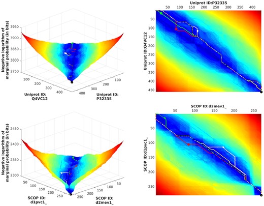
Landscapes generated for two randomly selected pairs, one pair taken from the Human ortholog benchmark, and the other from SABmark benchmark. For more, see Supplementary Section S5
3.2.2 Computational complexity and run times
The asymptotic time complexity to align any two sequences in our MML framework grows as . Any specific competing alignment can be probed and reported in time after the initial -effort to compute the marginal landscape. Using our distributed alignment program, the average run time required to compute and for a sequence pair from SABmark benchmark (on a standard Linux-based computer) is approximately 1.5 s and 1.7 s, respectively.
Acknowledgements
The authors thank Françios Petitjean for helpful suggestions on parameterizing Dirichlet distributions.
Funding
D.S.’s PhD scholarship is funded by Monash University. A.K.’s research is funded by Australian Research Council’s Discovery Project (DP150100894).
Conflict of Interest: none declared.
References

