


Abstract
The metabolites of exogenous and endogenous compounds play a pivotal role in the domain of metabolism research. However, they are still unclear for most chemicals in our environment. The in silico methods for predicting the site of metabolism (SOM) are considered to be efficient and low-cost in SOM discovery. However, many in silico methods are focused on metabolism processes catalyzed by several specified Cytochromes P450s, and only apply to substrates with special skeleton. A SOM prediction model always deserves more attention, which demands no special requirements to structures of substrates and applies to more metabolic enzymes.
By incorporating the use of hybrid feature selection techniques (CHI, IG, GR, Relief) and multiple classification procedures (KStar, BN, IBK, J48, RF, SVM, AdaBoostM1, Bagging), SOM prediction models for six oxidation reactions mediated by oxidoreductases were established by the integration of enzyme data and chemical bond information. The advantage of the method is the introduction of unlabeled SOM. We defined the SOM which not reported in the literature as unlabeled SOM, where negative SOM was filtered. Consequently, for each type of reaction, a series of SOM prediction models were built based on information about metabolism of 1237 heterogeneous chemicals. Then optimal models were attained through comparisons among these models. Finally, independent test set was used to validate optimal models. It demonstrated that all models gave accuracies above 0.90. For receiver operating characteristic analysis, the area under curve values of all these models over 0.906. The results suggested that these models showed good predicting power.
All the models will be available when contact with [email protected]
Supplementary data are available at Bioinformatics online.
1 Introduction
Cytochromes P450 (CYP450s) are the most important drug-metabolizing enzymes, most of which are oxidoreductases. Oxidoreductases are one of the main types of metabolic enzyme in organism. They play a vital role in the metabolism of both exogenous and endogenous compounds. As the most important biotransformation, it has been demonstrated that oxidation reactions catalyzed by oxidoreductases profoundly affect the effect of drugs and the metabolism of other xenobiotics (Zaretzki et al., 2011). Therefore, it is interesting to understand the metabolic profiles of xenobiotics.
As is known to all, the nature of the biotransformation is the break of old chemical bonds and the formation of new bonds in the presence of enzyme. Therefore, we defined the chemical bond within a molecule where the metabolic reaction occurred as site of metabolism (SOM). Information of SOM always plays an important role in the investigation of metabolic pathway of xenobiotics, and provides valuable information for the rational design and optimization of products. For example, drugs would undergo transformation and lead to two distinct consequences in the body. Metabolism of some drugs are likely to diminish or completely lose therapeutic efficacy, even lead to toxicity (Zimmerman and Maddrey, 1995). Some other drugs, however, tend to achieve better pharmacokinetic and bioavailability through metabolic transformation (Wiltshire et al., 2005). For the former, researchers can decide which sites on a molecule to modify in order to avoid undesired metabolism based on the information of SOM. The latter effect can be deliberately harnessed in the production of prodrugs that have favorable absorption properties but require metabolism to generate the therapeutically active compounds. Normally, the SOM is determined experimentally by metabolite identification techniques, such as HPLC-MS (Zhang et al., 2014). However, all such experimental techniques are time-consuming, and a computational model for SOM identification always allows chemists and pharmacologists to make rational decisions more quickly.
To date, there are various in silico models proposed for metabolism prediction, which adopt either ligand-based approaches or structure-based approaches (Kirchmair et al., 2012). Ligand-based approaches depend on the assumption that the metabolic fate of a compound is closely associated with its chemical structure characteristics (Melo-Filho et al., 2014). In ligand-based approaches, structures of known active and inactive compounds were used to develop prediction model (where ′activity′ refers to a measure of metabolism). There have been continuous attempts in the prediction of potential SOM by ligand-based methods, including rule-based methods (Marchant et al., 2008), pharmacophore-based methods (Jones et al., 1996), quantitative structure activity relationship (QSAR) methods (Li et al., 2008) and reactivity-based ab initio calculations (Liu et al., 2012). Although these ligand-based methods consume less time, the information of interaction between substrates and enzymes is not considered. Thus, these ligand-based methods fail to give a rational result about regioselectivity of substrates (Dai et al., 2014). Structure-based approaches simulate the process of enzyme-substrate complex formation. Both the ligand, the protein and the ligand–protein complex are considered (Tarcsay and Keseru, 2011). To perform structure-based metabolism prediction, three-dimensional (3D) structures of the metabolic enzymes are required. However, 3D structures of many enzymes are unclear. In addition, as the most significant drug-metabolizing enzymes, CYP450s exhibit poor specificity to their substrates (Hendrychova et al., 2011; Sheng et al., 2014). All these factors seriously impede the application of structure-based approaches to determine the SOM. To accurately predict the SOM of a series of CYP2C9 substrates, Kingsley et al. (2015) outlined a novel approach combining ligand- and structure-based design principles. Although this approach provided some useful information about the potential SOMs mediated by CYP2C9, it is hard to make further progress without 3D structures of metabolic enzymes.
To sum up, most in silico methods are only focused on metabolism mediated by several specified CYP450s. Although CYP450s are the most important drug-metabolizing enzymes, they are not the only ones. We cannot ignore the roles of other metabolic enzymes in the process of drug metabolism. In addition, many models only apply to substrates with special skeleton (Dai et al., 2015), which have poor transferability. When a model has no restrictions on the structures of substrates, we consider it has good transferability. Otherwise, it will be regarded as poor transferability.
Only considering quantum chemical (QC) features of the SOM, Zheng et al. developed a model for determining SOM in the presence of only CYP3A4, 2C9, and 2D6 by incorporating the use of machine learning and semiempirical quantum chemical calculations, which gave an accuracy of approximately 0.80 for external test (Zheng et al., 2009). It should be pointed out that neither MetaSite (combining structure- and ligand-based approaches) (Cruciani et al., 2005) nor the model (QSAR-models) built by Sheridan et al. (2007) can explain more than about 70% of the regioselectivity data for the same external test. It indicated that it is promising to predict the reactivity for substrates based on QC of the SOM.
In this work, SOM prediction models for six biotransformations mediated by oxidoreductases were developed from the integration of enzyme data and chemical bond information by the use of machine learning. First, an optimum database was obtained by investigating 11 metabolic reaction databases. Then physicochemical properties and topological properties for every SOM in the substrate were calculated to describe the characteristics of each SOM in combination with the corresponding enzymes, and these properties were used as input to train classifiers. Reaction type of each SOM was marked manually by comparing each pair of reactant and product structures. Finally, six types of oxidation reaction mediated by oxidoreductases were considered. A variety of feature selection algorithms (CHI, IG, GR, Relief) were implemented to train the prediction models, in combination with multiple classification procedures (KStar, BN, IBK, J48, RF, SVM, AdaBoostM1, Bagging). As a result, four series of prediction models for each reaction were acquired. Optimum models were obtained through a comparison among these models. For validation, the proposed methods were tested by the independent test set.
2 Methods
2.1 Datasets
High-quality data helps modeling successfully. To select a suitable data source, 11 metabolic reaction databases were investigated. We evaluated their accuracy, completeness and applicability through exploring their original data source, number of metabolic reactions and data format, respectively. The details were described in Table 1. It should be noted that the database of which data derived from the literature was taken into consideration, with maximum number of metabolic reactions and high applicability. As a result, BKM-react, an integrated biochemical reaction database, was selected as an optimum database. BKM-react comprises 28 042 unique biochemical reactions, as source databases the biochemical databases BRENDA, KEGG and MetaCyc were used. In addition, all reactions in BKM-react were collected from the literature or experiment (Lang et al., 2011).
Overview of descriptive statistics of 11 metabolic reaction database
| Database | Site | Accuracy | Completeness | Applicability |
|---|---|---|---|---|
| KEGG | http://www.kegg.jp/ | Literature | 10 049 | High |
| HMDB | http://www.hmdb.ca/ | Literature | 6302 | High |
| HumanCyc | http://humancyc.org/ | Literature | 2368 | High |
| HMR | http://www.metabolicatlas.org/ | Literature | Over 8000 | High |
| BKM-react | http://bkm-react.tu-bs.de/ | Literature | 28 042 | High |
| Sabio-rk | http://sabio.h-its.org/ | Literature | 6867 | High |
| Drugbank | http://www.drugbank.ca/ | Literature | 1405 | High |
| BioPath | http://www.molecular-networks.com/databases/biopath | Literature | 3900 | High |
| Kpath | http://browser.kpath.khaos.uma.es/ | Literature | 13 153 | High |
| SMPDB | http://smpdb.ca/ | Literature | 1718 | High |
| Reactome | http://www.reactome.org/ | Literature, Prediction | 70 361 | Medium |
The generation procedures of datasets used in the present research were shown below:
Reactions mediated by oxidoreductases were taken into consideration;
The 3D structures of reactants and products were exported from BKM-react;
Reactants of all the reactions retrieved were filtered based on atom-type content, only C, H, O, N, S, P, F, Cl, Br and I were permitted. Then potential SOMs and the reaction type of SOMs were marked manually by comparing each pair of reactant and product structures. Enzymes catalyzing the corresponding reactants were recorded simultaneously to represent the interaction between SOMs and enzymes. Every SOM was marked by keeping a record of atomic indices of the two atoms located at either end of the chemical bond where biotransformation occurred. Equivalent bonds are marked identically. Every chemical bond is a potential SOM, only SOMs observed experimentally were regarded as positive SOMs (labeled as ‘1’). In contrast, if a SOM has not been detected as a positive SOM, we regarded it as non-positive SOM, it was marked as an unlabeled SOM (labeled as ‘0’). Then, all of the SOMs were categorized according to their reaction types. Finally, six classes of reaction mediated by oxidoreductases were considered to develop SOM prediction models. Visual graphic definitions of these reactions were listed in Table 2. The description of positive SOMs, unlabeled SOMs and the corresponding enzymes were detailed in the Supplementary file S2. Structures of compounds were available in Supplementary file S3.
Table 2Visual graphic definitions of six reactions mediated by oxidoreductases
ID Name Definition I Alcohol Oxidation to Ketone 
II Alcohol Oxidation to Aldehyde 
III Carbon Doublebond Formation 
IV Oxidative Deamination 
V N-Dealkylation 
VI Hydroxylation 

ID Name Definition I Alcohol Oxidation to Ketone II Alcohol Oxidation to Aldehyde III Carbon Doublebond Formation IV Oxidative Deamination V N-Dealkylation VI Hydroxylation SOM of each reaction type was marked with dashed circles.
Table 2Visual graphic definitions of six reactions mediated by oxidoreductases
ID Name Definition I Alcohol Oxidation to Ketone II Alcohol Oxidation to Aldehyde III Carbon Doublebond Formation IV Oxidative Deamination V N-Dealkylation VI Hydroxylation ID Name Definition I Alcohol Oxidation to Ketone II Alcohol Oxidation to Aldehyde III Carbon Doublebond Formation IV Oxidative Deamination V N-Dealkylation VI Hydroxylation SOM of each reaction type was marked with dashed circles.
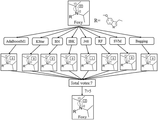
In this step, negative SOMs (SOMs where biotransformation can’t occur) were attained by screening the unlabeled SOMs. The screening procedures were detailed as follows. First, positive SOMs and unlabeled SOMs attained from step 3 were utilized to establish discriminative models by eight effective classification procedures (KStar, BN, IBK, J48, RF, SVM, AdaBoostM1, Bagging). Consequently, eight discriminative models were obtained. Then, each unlabeled SOM was assigned a score depending on the discriminative results. When an unlabeled SOM was determined to be unlabeled by one discriminative model, the unlabeled SOM got 1 score, otherwise 0 score was recorded. Finally, a voting method was used to determine whether an unlabeled SOM is negative SOM or not. Here, scores of each unlabeled SOM were aggregated. We defined the unlabeled SOMs of which score > 5 as negative SOMs (labeled as ‘-1’). All the results were derived from a 10-fold cross-validation (10-CV).
Such a screening procedure for the case of Foxy (a molecule) was demonstrated in Figure 1. The bond N12-C13 of Foxy is a SOM which has not been detected experimentally as a positive SOM. Therefore, we regarded it as an unlabeled SOM. Then eight discriminative models attained above were utilized to predict N12-C13 is an unlabeled SOM or a positive SOM. It turned out that only the J48 model determined N12-C13 as a positive SOM, and the remaining seven models predicted N12-C13 as an unlabeled SOM. According to the scoring principles mentioned above, N12-C13 scored 7 in total. Therefore, N12-C13 was regarded as a negative SOM in the current study. For other unlabeled SOMs, the same screening procedure was conducted.
For SOMs catalyzed by certain enzyme, only both positive SOMs and negative SOMs recorded in our datasets were retained, if either positive SOMs or negative SOMs were absent, the SOMs mediated by this enzyme were discarded to minimize the risks of sample imbalance.
Dataset of each reaction type was randomly divided into training and test set in the ratio of 4:1. Descriptive statistics of these datasets were shown in Table 3.
The identification procedure of negative SOMs of an example chemical. 1, 0, and -1 (in the small box) represent positive SOM, unlabeled SOM and negative SOM, respectively
Descriptive statistics of SOM datasets of six reactions mediated by oxidoreductases
| Reaction type | NO of SOM | NO of compounds | NO of enzymes | |||
|---|---|---|---|---|---|---|
| Unlabeled | Positive | Negative | Sum | |||
| I | 1907 | 651 | 1678 | 2329 | 483 | 269 |
| II | 481 | 142 | 440 | 582 | 221 | 71 |
| III | 2129 | 708 | 1897 | 2605 | 317 | 123 |
| IV | 179 | 103 | 138 | 241 | 87 | 23 |
| V | 302 | 86 | 250 | 336 | 104 | 38 |
| VI | 2438 | 861 | 2112 | 2973 | 372 | 218 |
The description of positive SOMs and negative SOMs were detailed in Supplementary file S4.
2.2 Descriptors of chemical bond
Computational description is necessary to in silico prediction. To carry out computational description of the chemical bond, descriptors of chemical bond were considered, which have been used to predict the classification of photochemical reactions (Zhang and Aires-de-Sousa, 2005). In this work, 56 descriptors of chemical bond were calculated based on Hückel molecular orbital method, mulliken charge analysis, hybrid orbital theory and valence-bond theory, including 29 physicochemical properties and 27 topological properties. The properties were detailed in Supplementary Table S1 (see Supplementary file S1).
Physicochemical properties considered in this paper mainly describe properties associate with the partial charge distribution which determines many features of a molecule, such as, ionization constants, electron affinity and pharmacophore pattern. Many of these features have been proposed to explain the chemical selectivity or reactivity of a compound (Kolandaivel et al., 2005). All the properties were calculated by the quantum chemistry program Marvin (https://www.chemaxon.com/).
For topological descriptors, both hybridization state of atoms located at either end of the chemical bond and bond order were considered. Bond order characterizes the strength and stability of a chemical bond. We also took the information of atoms adjacent to atoms located at either end of the chemical bond into consideration. By doing so, we attempt to describe the chemical environment of SOM as accurately as possible.
2.3 Feature selection and classifier
2.3.1 Feature selection
Feature selection (FS) is a method which provides optimal classification accuracy of the discriminative model by selecting an optimal and minimal set of features (Saeys et al., 2007). During the last decade, FS has shifted from an illustrative example to a real prerequisite for modelling. To prevent classification of noise and redundant information, four FS algorithms (CHI, IG, GR, Relief) shown effective in many applications were adopted. The descriptions of these methods were detailed in Table 4.
Overview of FS algorithms and classifier algorithms
| Name | Full name | Description | Refs. |
|---|---|---|---|
| CHI | ChiSquared | Evaluates the worth of an attribute by computing the value of the chi-squared statistic with respect to the class, and provides a feature ranking as a result | Hernández-Torruco et al. (2014) |
| GR | GainRatio | Reveals the association between an attribute and the class value by measuring the gain ratio of each attribute with respect to the class. The higher the gain ratio, the more significant for the instance categorization the attribute | Ramani and Jacob (2013) |
| IG | InfoGain | Evaluates the worth of an attribute by measuring the information gain with respect to the class. The idea is to estimate the difference between the prior entropy of class C and posterior entropy. Finally, a feature ranking was provided | Zheng et al. (2004) |
| Relief | Relief | Evaluates the worth of an attribute by repeatedly sampling an instance and considering the value of the given attribute for the nearest instance of the same and different class. Consequently, a feature ranking was given. The key idea is to estimate attributes according to how well their values distinguish among instances that are near each other. The rationale is that a good attribute should differentiate between instances from different classes and should have the same value for instances from the same class | Kononenko (1994) and Pang et al. (2015) |
| AdaBoostM1 | AdaBoostM1 with C4.5 decision tree as its base-level classifier | The purpose of AdaBoostM1 is to find a highly accurate classification rule by combining many weak classifiers, each of which may be only moderately accurate. The weak classifiers are learned sequentially, one at a time. Conceptually, at each iteration the weak classifier is biased to classify the examples which were most difficult to classify by the preceding weak classifiers. After a certain number of iterations, the resulting weak classifiers are linearly combined into a single rule. In the current study, AdaBoostM1, an ensemble method, was used with C4.5 decision tree as its base-level classifier | Shang (2014) and Romero et al. (2004) |
| KStar | KStar | KStar, an instance-based classifier, is based on K-nearest neighbors framework, and its basic idea is to measure the difference between input samples and pre-classified instances by using entropy-based distance. For this method, the distance between instances is defined as the complexity of transforming one instance into another. In the category prediction, the probability of an instance a being in category C was calculated by summing the probabilities from a to each instance that is a member of C. The probabilities for each category are calculated. The category with the highest probability is selected as the category of the new instance | Cleary and Trigg (1996) and Ozcift (2012) |
| BN | Bayes | This classifier learns from training data, the conditional probability of each attribute Ai given the class label C. Classification is then done by applying Bayes rule to compute the probability of C given the particular instance of A1, . ., An, and then predicting the class with the highest posterior probability | Pernkopf and Wohlmayr (2013) |
| IBK | K-nearest neighbours | The IBK classifier is commonly based on the Euclidean distance between a test sample and the specified training samples. The classification rule is to assign a test sample to the majority category label of its k nearest neighbors | Chavan et al. (2014) |
| J48 | C4.5 Decision Tree | This classifier is generated based on the instances, and focuses on deducing classification rules represented by decision tree from a group of out-of-order or out-of-rule samples. C4.5 algorithm is developed by improving the ID3 algorithm. It uses gain ratio impurity method to evaluate the splitting attribute. At each node of the tree, C4.5 chooses one of the data that most effectively splits its set of samples into subsets enriched in one class or the other. Its criterion is the normalized information gain that results from choosing an attribute for splitting the data. The attribute with the highest normalized information gain is chosen to make the decision | Quinlan (1986) and Hu et al. (2012) |
| RF | RandomForest | Random forest classifiers work by growing a predetermined number of decision trees simultaneously. A test instance is run on all the decision trees grown in the forest. Each tree’s classification of the test instance is recorded as a vote. The votes from all trees are aggregated and the test instance is assigned to the class that receives the maximum votes | Jayaraj et al. (2016) |
| SVM | Support Vector Machines | Input vectors are non-linearly mapped to a very high-dimension feature space. Where a linear decision surface is constructed. The goal of the SVM algorithm is to find an optimal hyperplane that separates the training samples by a maximal margin, with all positive samples lying on one side and all negative samples lying on the other side based on statistical learning theory. In this work, LibSVM, an effective SVM method, was adopted | Chang and Lin (2011) |
| Bagging | Bagging with KNN as its base-level classifier | Bagging predictors is a method for generating multiple versions of a predictor based on re-sampling techniques and using these predictors to get an aggregated predictor. The multiple versions are formed by making bootstrap replicates of the learning set and using these as new learning sets. Finally, a voting method was used to determine the final prediction function. In the current study, Bagging with KNN as its weak classifier was adopted to develop predictive model | Breiman (1996) and Ashtawy and Mahapatra (2015) |
2.3.2 Classifier
Machine learning systems are systems that learn from known data and attempt to recognize characteristic patterns (Gruss et al., 2015). After a ′training phase′, a predictive model will be returned which can be used to map unknown input data into a category. Generally, establishing discriminative model is the preferred method to handle a two-class problem. So far there are various classifiers reported, each of which has their own strength and weakness. There is no classification algorithm which outperformed other classification procedures in all domains. To select optimal method for each type of reaction, eight classification algorithms (KStar, BN, IBK, J48, RF, SVM, AdaBoostM1, Bagging) were considered in the current study, which are effective in various domains of bioinformatics and medicinal chemistry. All these methods were detailed in Table 4.
To obtain optimal discriminative model, a FS-Classifier strategy was adopted, and it was accomplished by four FS algorithms, in combination with eight classification procedures. Then a comparison among these combinations was conducted. The workflow of the selection of optimal models by the FS-Classifier strategy was demonstrated in Figure 2.
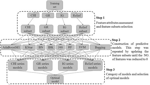
The workflow of screening optimal model based on FS-Classifier strategy
Step 1: Four FS methods were utilized to select feature subset. All of these FS algorithms are focused on assigning a significant score to each feature attribute, and ranking these feature attributes in descending order. A higher score represents the feature is more significant for the training categorization. Features scoring 0 were regarded as redundant and discarded. The remaining features were retained as feature subsets.
Step 2: Eight classifier procedures were used to establish predictive models based on feature subsets. This step was repeated by updating the feature subsets until the number of features reduced to 0, which started with the result feature subsets obtained from step 1, and eliminated the feature with the lowest score in the next round.
Step 3: All the models attained in step 2 were divided into four categories according to the FS methods. Consequently, four series of models were achieved for each type of reaction. A comparison among the predictive models was conducted for each biotransformation. The model which gave the highest ACC and gave an area under curve (AUC) > 0.9 was selected as the optimal model. The goodness of a feature subset was assessed by the performance of the classifier. Thus, the optimal feature subset for each biotransformation was also attained in the current Step.
The above mentioned FS-classifier strategy was implemented in Waikato Environment for Knowledge Analysis (WEKA) data mining environment (Mark Hall, 2009). All the FS techniques and classification procedures were taken place within 10-CV. All the parameters and configurations of the programs were set to default values provided by the WEKA data mining environment.
2.4 Prediction quality measurement
To give further information about the performance of these models. Also, receiver operating characteristic (ROC) analysis was carried out. In this step, AUC was calculated as a measure of the quality of the SOM prediction models. Commonly, the AUC value ranges from 0.5(random classifier, no predictive value) to 1.0 (ideal classifier, perfect prediction). A higher AUC value means the model is more reliable (Linden, 2006).
3 Results
3.1 Selection of optimal models
According to the method shown in Figure 2, four series of models for each reaction type were developed. To select optimal model for each reaction type, comparisons among these models were performed. The model that gave the highest value of ACC and gave an AUC value above 0.9 was selected as optimal model.
Figure 3 demonstrated such a selection procedure for the case of N-dealkylation. The results suggested that optimal model was attained by the combination of KStar and Relief when the feature number was declined to 26. For other reaction types, the same process was conducted. Consequently, optimal model for each biotransformation was obtained (Table 5). The feature number of each optimal model ranged from 8 to 26 except for Carbon Doublebond Formation that gave a feature number of 45, which revealed that all of these models were simplified.
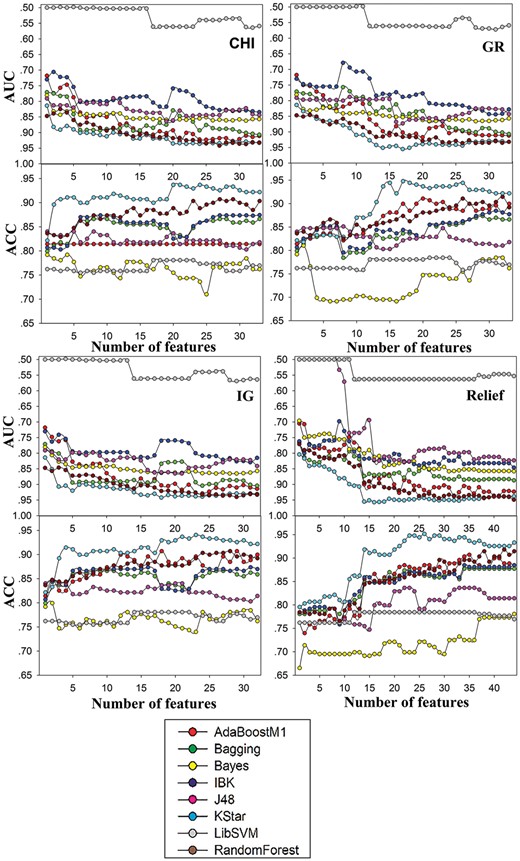
Four series of models for N-Dealkylation (CHI series, GR series, IG series, Relief series). Plots to compare different combinations of FS algorithms and classifier algorithms, where both the ACC and AUC derived from 10-CV are plotted as functions of the number of features. Different classification methods were characterized with different colors
Optimal models selection results
| Type | Classifier | FS | No. of features |
|---|---|---|---|
| I | KStar | CHI/IG | 12 |
| II | KStar | CHI/GR/IG | 10 |
| III | RandomForest | IG | 45 |
| IV | KStar | CHI/GR/IG | 8 |
| V | KStar | Relief | 26 |
| VI | KStar | CHI | 12 |
| Type | Classifier | FS | No. of features |
|---|---|---|---|
| I | KStar | CHI/IG | 12 |
| II | KStar | CHI/GR/IG | 10 |
| III | RandomForest | IG | 45 |
| IV | KStar | CHI/GR/IG | 8 |
| V | KStar | Relief | 26 |
| VI | KStar | CHI | 12 |
Among all the combinations, the combination of KStar and CHI appears the best because it gave the best performance for four of the problems studied followed by the combination of Kstar and IG which gave the best performance for three. We can also conclude that there is a difference among the optimal combinations of FS algorithms and classifier algorithms for different reaction types. These results reflected that it seems to be an effective method to establish optimal model through a variety of FS algorithms, in combination with multiple classification procedures.
The features which were used to develop model for each biotransformation were demonstrated in Figure 4, from which we can easily find that it consisted of physicochemical properties and topological properties for each reaction type. However, the subsets of Alcohol Oxidation to Ketone and Alcohol Oxidation to Aldehyde only contained physicochemical properties. These results may be a direction that it is closely related to the physicochemical properties of chemical bonds for Alcohol Oxidation reaction.
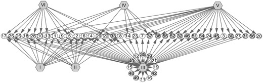
A network to show which descriptors were utilized in the models. Gray hexagons represent the six models established in the current study. Gray circles represent topological properties, white circles represent physicochemical properties. ID in circles corresponds to ID in table 1S. The edge between a circle and a hexagon indicates the property was contributed to the construction of the corresponding model
Note that four physicochemical properties qsigma_A (ID: 2), oensigma_A (ID: 5), doensigma (ID: 28) and doenpi (ID: 29) may be more closely associated with the regioselectivity of substrates than others, which were included in five subsets among six feature subsets. It should be noted that all the four features mentioned above are related to A, however, only the last two are associated with B. Probably, all of the B are hydrogens for Alcohol Oxidation to Ketone, Alcohol Oxidation to Aldehyde and Hydroxylation. These discoveries may provide some valuable information for determining important features when oxidoreductases mediated SOM prediction models are developed.
3.2 Performance measurements
The overall performance of each prediction model was measured by multiple indices (Table 6). The ACC of training set ranged from 0.904 to 0.995, the AUC ranged from 0.915 to 0.999, SE and SP were generally in excess of 0.875 and 0.949, respectively, except for Hydroxylation (equal to 0.795 ) and Alcohol Oxidation to ketone (equal to 0.777). For validation, the ACC for each prediction model exceeded 0.904 while the SP was 0.956 to 1, and the SE for every model was greater than 0.826 except for Alcohol Oxidation to ketone (equal to 0.777) and Hydroxylation (equal to 0.774). In terms of BACC, both the training set and test set gave the values >0.865. These results demonstrated that our method is quite effective for the construction of prediction model.
Prediction quality of the six optimal SOM models for 10-CV prediction and independent test set prediction
| Dataset | Type | SE | SP | ACC | BACC | AUC |
|---|---|---|---|---|---|---|
| I | 0.777 | 0.975 | 0.921 | 0.876 | 0.962 | |
| Trainning set | II | 0.899 | 0.968 | 0.951 | 0.934 | 0.979 |
| III | 0.909 | 0.989 | 0.967 | 0.949 | 0.989 | |
| IV | 0.988 | 1 | 0.995 | 0.994 | 0.999 | |
| V | 0.875 | 0.976 | 0.952 | 0.926 | 0.943 | |
| VI | 0.795 | 0.949 | 0.904 | 0.872 | 0.915 | |
| I | 0.777 | 0.963 | 0.908 | 0.87 | 0.963 | |
| Test set | II | 0.826 | 0.989 | 0.957 | 0.908 | 0.985 |
| III | 0.903 | 0.995 | 0.969 | 0.949 | 0.986 | |
| IV | 0.95 | 1 | 0.979 | 0.975 | 1 | |
| IV | 0.909 | 0.978 | 0.955 | 0.944 | 0.987 | |
| VI | 0.774 | 0.956 | 0.904 | 0.865 | 0.906 |
Almost each model performed well, of which all their indices were over 0.875. However, the performance of Hydroxylation and Alcohol Oxidation to ketone were not as good as others. Such a result may be attributed to the relatively complicated mechanism. Generally, the reaction mechanism of Hydroxylation can be summarized as hydrogen abstraction or oxygen rebound (Groves and McClusky, 1978). Hydroxylation was often accompanied by the generation of intermediate. Of course, direct Hydroxylation can also occur. Such a complicated mechanism leads to a low specific SOM pattern. Another challenge to define SOM of Hydroxylation is that our model contained metabolism information of aliphatic C-hydroxylation and aromatic C-hydroxylation, which raised the prediction difficulty.
ROC analysis has become increasingly popular over the past few years as a method to judge the discrimination ability of various statistical methods. It is considered as an effective method to assess the reliability of a discriminative model. ROC curves for our six prediction models on their respective test dataset were demonstrated in Figure 5. A random classifier would return a point along the diagonal line (broke line in red). Conversely, an ideal classifier would give a point in the upper left corner of the ROC space. It is not hard to notice that all of the ROC curves were approaching the perfect prediction point. The AUC of each ROC curve was given in Table 6, from which we can find each of our model gave a significant AUC value >0.963. Also, there was an exception that Hydroxylation gave a value of 0.906. These statistical results further confirmed the reliability of our models.
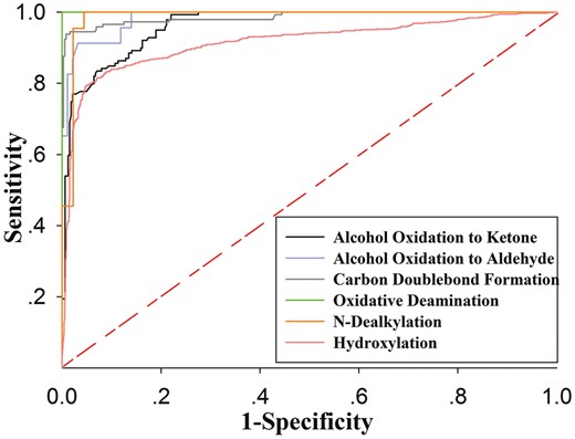
ROC curves of SOM prediction models for six reactions mediated by oxidoreductases on their respect internal test
4 Discussion
We have established SOM prediction models for six oxidoreductases-mediated reactions. Obviously, structure-based methods were not used in this paper. However, it should be noted that our method is significantly different from ligand-based approaches. Our models were established on the scale of chemical bond instead of molecular. Therefore, they exhibited stronger generalization ability compared with those models which are only focused on compounds with special skeleton. In other words, there is no limit to the structures of substrates for the scope of application of our models. Therefore, we can claim that our models have good transferability.
Generally, ligand-based approaches always fail to take the interaction between enzymes and substrates into account. Therefore, these models can predict only where a molecule might be oxidized assuming it is a substrate of certain enzyme, which always leads to results with lower explanation (Sheridan et al., 2007). To address this issue, an effective method is to treat SOM and the corresponding enzyme as a system. In this paper, when a potential SOM is experimentally observed, we considered it and the corresponding enzyme as a positive system (the potential SOM can occur biotransformation in the presence of the corresponding enzyme). In contrast, it will be regarded as an unlabeled system (the potential SOM is an unlabeled SOM in the presence of the corresponding enzyme) where negative system (the potential SOM can’t occur biotransformation in the presence of the corresponding enzyme) was filtered. Finally, discriminative models were developed based on the positive systems and the negative systems. By doing so, we considered not simply reactivity for molecules but binding properties between enzymes and substrates. There is no doubt that a more reasonable result can be attained by the method proposed above.
Unlike other SOM prediction models which classified the SOMs not reported in literature as negative SOMs directly (Zheng et al., 2009), our method offered a more reasonable classification by dividing all potential SOMs into positive SOMs and unlabeled SOMs. Negative SOMs were acquired by screening the unlabeled SOMs. The reasons we hold the view that non-positive SOMs in the datasets should be classified as unlabeled SOMs instead of negative SOMs are as follows: on the one hand, some real SOMs may have not been successfully recognized in experiments, many new reactions are discovered with the rapid development of detection technology. On the other hand, some SOMs of reactants in our datasets may not be recorded although we have selected the optimum database. After all, there is no database collecting all the reactions observed in experiments so far. The quantity of false negative samples will increase if we labeled SOMs without recorded in the literature as negative SOMs directly. By doing so, we attempt to minimize the risks brought by false negative samples. Another advantage of the method is the utilized of the FS-Classifier strategy, aimed at attaining the optimal combination of FS and classifier through filtering the combinations of a variety of FS algorithms and multiple classification procedures.
The data on reaction of enzymes were derived from different organisms (including human, intestinal bacteria, microorganisms and some plants). How such a multi-species source enzyme data may help in the prediction of SOMs in the human body? In fact, our models were established only rely on the interaction between SOM and enzyme. We have not taken in vivo environment into consideration. Therefore, our model can’t completely simulate the metabolism of exogenous compounds in the human body. It should be noted that the object of this article is not to simulate the in vivo metabolism of drugs, but to predict in vitro metabolism of exogenous compounds in the presence of enzyme. Then, we can infer the metabolism of exogenous compounds in the human body based on our in vitro prediction results. In other words, the model established in the present study is an in vitro prediction model, this in vitro prediction model is only associated with SOM and enzyme. There is no relation between our models and the species of which the enzyme exists. We acknowledge that we fail to take in vivo environment of the organism into consideration. However, it should be noted that all the prediction models reported were established based on metabolism data which were attained from in vitro enzyme catalysis experiment, they also failed to take in vivo environment into consideration. We believe such a situation will not changes until more advanced identification techniques are proposed.
How our models to predict the metabolism of exogenous compounds in the human body? As mentioned above, our models not only output metabolites but also provide information about the enzyme which catalyzes the metabolism. Therefore, we can infer the in vivo metabolism of exogenous compounds rely on whether the enzyme exists in the human body. If an enzyme exists in the human body, we think the corresponding metabolites will exist in the human body, otherwise, the corresponding metabolites will not exist in the human body.
In summary, this work presents a novel method to infer SOM for biotransformations mediated by oxidoreductases by the integration of chemical bond data and enzyme information based on a FS-Classifier strategy. Meanwhile, a new concept of the model’s transferability was proposed. By incorporating the use of machine learning and quantum chemical calculations, SOM prediction models for six reactions mediated by oxidoreductases were established on the level of chemical bond. Both 10-CV and independent test set validation results indicated that the models were considerable success. We believe our models will assist in the process of lead optimization in the early stage of drug discovery and development. Also, they will provide valuable information for research on enzyme bioconversion system (in industry, enzyme bioconversion system is widely used in the production of bioconversion products).
The performance of our method may be improved by adopting more appropriate parameters in practical application. Therefore, our future works will target on the development of appropriate parameter optimization. Furthermore, a web service for SOM estimating and visualizing will be built. SOM prediction models for other reaction types mediated by oxidoreductases or other types of metabolic enzymes will make a significant breakthrough when sufficient data is available.
Funding
This work has been supported by the National Natural Science Foundation of China (grants 81173568, 81373985, and 81430094), Program for New Century Excellent Talents in University (Grant NCET-11-0605).
Conflict of Interest: none declared.
References

