


Abstract
Recent technological advances in high-throughput sequencing and genotyping have facilitated an improved understanding of genomic structure and disease-associated genetic factors. In this context, simulation models can play a critical role in revealing various evolutionary and demographic effects on genomic variation, enabling researchers to assess existing and design novel analytical approaches. Although various simulation frameworks have been suggested, they do not account for natural selection in admixture processes. Most are tailored to a single chromosome or a genomic region, very few capture large-scale genomic data, and most are not accessible for genomic communities.
Here we develop a multi-scenario genome-wide medical population genetics simulation framework called ‘FractalSIM’. FractalSIM has the capability to accurately mimic and generate genome-wide data under various genetic models on genetic diversity, genomic variation affecting diseases and DNA sequence patterns of admixed and/or homogeneous populations. Moreover, the framework accounts for natural selection in both homogeneous and admixture processes. The outputs of FractalSIM have been assessed using popular tools, and the results demonstrated its capability to accurately mimic real scenarios. They can be used to evaluate the performance of a range of genomic tools from ancestry inference to genome-wide association studies.
The FractalSIM package is available at http://www.cbio.uct.ac.za/FractalSIM.
Supplementary data are available at Bioinformatics online.
1 Introduction
The rapid growth of genomic technologies has generated high-throughput omic data and enhanced the development of a range of statistical genomic approaches ranging from ancestry inference to disease scoring statistics, to analyse and handle these large-scale data. Accuracy, effectiveness and performance assessments of different analytical methods used to analyse genetic data are crucial aspects of medical population genetics.
The identification and characterization of the ancestry of single nucleotide polymorphisms (SNPs) and SNPs that confer increased susceptibility to complex human diseases are central research area in genomics. However, there is in general, no ground-truth knowledge of SNP ancestry or SNPs which are actually disease causing when deploying ancestry inference methods or novel genome-wide association studies (GWAS) in real data. Therefore to facilitate genomic studies, genomic data simulators with more sophisticated capabilities and features need to be implemented (Yuan et al., 2012) and made publicly available. Simulation studies and their availability to genomics communities may improve our understanding of the impact of various evolutionary, admixture and demographic scenarios on genomic variation and permit adequate assessment of existing tools and design of novel analytical methods (Yuan et al., 2012).
Genomic sequences are exposed to genetic pressures and complex environmental factors, which have not been considered in most currently available simulation frameworks. Currently several genomic simulation tools exists (Escalona et al., 2016), including HAPGEN2 (Su et al., 2011) and SIMCOAL 2.0 (Laval and Excoffier, 2004), which are based on resampling approach models and identified as being the best in conserving the Linkage Disequilibrium (LD) structure of the input datasets. Most of these simulation tools are based on a particular chromosome or a specific genome region. Mimicking the genome-wide by exploring various evolutionary models in a single simulation framework, that integrates a range of genetic models such as natural selection in admixture scenarios and epigenetic interactions, will improve modelling accuracy and genomic tool assessment.
In this article, we present a multi-scenario genome-wide simulation framework, FractalSIM (Fig. 1). It has the capability to accurately mimic and generate genome-wide data under various genetic models of genetic diversity and genomic variation affecting diseases in admixed and/or homogeneous population, particularly those under natural selection. The framework accounts for natural selection pre-and post-admixture processes. With FractalSIM, we successfully simulated genome-wide data for a variety of mixed ancestry populations and different scenarios. Tools showed promising results in mimicking real datasets when assessed by current tools used in ancestry inference and GWAS. FractalSIM will, therefore, be useful for the evaluation of current and future analytical methods in genomics.
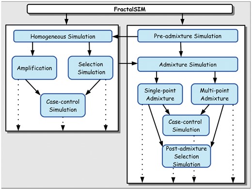
Overall workflow of FractalSIM tool. The bold arrows indicate possible options for simulation, and the dotted arrows indicate possible outputs from FractalSIM
2 Materials and methods
2.1 Simulation of population bottleneck
2.2 Population bottleneck under selection
FractalSIM allows users to implement either negative, positive or balanced selection pressure. Users may specify the SNPs under selection and the relative fitness of carrying 1 or 2 copies of the minor allele, relative to carrying 2 copies of the reference allele, depending on the required selection pressure. Let S be the number of SNPs specified under selection, and be the number of minor alleles at SNP j, for two adjacent haplotypes, corresponding to a given individual. Let fj be the relative fitness of gj, thus the overall fitness of the individual, denoted F, is obtained under the multiplicative selection model as . Let . The conditional probability of an offspring to survive given g, . There are 3S possible genotypes permutations of the SNPs specified under selection. Let Fi be the overall fitness of permutation i, and be the set that contains the two highest overall fitness. We refer to T as the threshold set. FractalSIM applies the rejection-sampling method as described in Peng et al. (2012), by implementing an object that obtains the set T, and an offspring only survives if its overall fitness is in T.
The simulation proceeds in pairs of consecutive haplotypes (corresponding to an offspring genotype), hR+1 and hR+2. The distinct segments are first simulated as discussed in Section 2.1. The set g for an offspring, whose overall fitness is in T, is then obtained. Here the aim is to simulate an offspring with the set g of genotypes at the SNP positions under selection. Each is then separated according to the number of minor alleles as . The copying state for a simulated segment of hR+1 that contains SNP j under selection, is only accepted if it contains at SNP j. Similarly for haplotype hR+2, the copying state of the segments that contain SNP j is only accepted if it contains at SNP j. To reduce the computational cost involved in this step, S clusters are formed, each containing all the copying states. Each cluster is assigned a SNP under selection, and further partitioned into two sets of the copying states depending on whether the haplotype corresponding to a copying state has 0 or 1 at the corresponding SNP under selection. Depending on value of and , we used random sampling to extract the copying states from a given set of segment containing a SNP to be simulated under selection. The copying states for the segments with no SNP under selection are extracted as described in Section 2.1. Genotyping and mutation processes are implemented as in Section 2.1 for all the segments.
2.3 Case-control under population bottleneck
Users may opt to simulate a case-control null or causal model. The causal model is determined by the relative risks that users specify, corresponding to carrying either one or two copies of minor allele as the risk allele. The datasets generated may be used in the assessment of association methods to ascertain false positive and/or false negative results.
In step 1, we determine D for all the cases and controls. Step 2 involves the simulation of the crossover positions, which is obtained similarly to Section 2.1. In step 3, the exact copying states are determined. The copying state of the segments without a risk allele is determined as in Section 2.1. Similarly to Section 2.2, we obtain the copying state for the segments that contains the risk SNPs. Defining the genotype at each di as , then di is first split according to the number of minor alleles as . The copying state for a segment in hR+1 that contains SNP i is only accepted if it contains at SNP i, while the copying state of the segment of hR+2 is only accepted if it contains at SNP i. To reduce the computation cost for this step we proceed as in Section 2.2, but creating I clusters corresponding to each risk SNP i. In step 4, genotypes are then copied to the simulated segments following a mutation process as in Section 2.1 in step 4. The copying state and the genotype for haplotype hR+2 are obtained in a similar manner. Steps 2–4 are then repeated until all the cases and controls specified are simulated. The generated case and control haplotypes are output in two different files.
2.4 Multi-way admixed population
FractalSIM can simulate a K-way admixture scenario for any K ≥ 2 and considers two scenarios in the simulation of admixture including single-point admixture or multi-point admixture. In a single-point scenario all the parental populations interbreed at one point in history, and in subsequent generations breeding occurs only within the admixed population with no further contribution from the ancestral populations. To implement these scenarios, the breaking points between the discrete chromosomal chunks are modelled using a Poisson distribution at a given rate per unit genetic distance.
In a multi-point admixture simulation, we consider a scenario with a continuous flow of ancestry in the history of the admixed population. The model mimics the scenario that few ancestral populations met and interbred at a certain generation and over time other ancestral populations interbreed with the hybrid population, at given generations, which constitutes the final hybrid population. FractalSIM receives a parameter file specifying the continuous flow of ancestral populations with additional information pertaining to the above simulation. In the first instance, FractalSIM implements the first single-point admixture scenario. In subsequent points of admixtures it treats the previously simulated admixed population as one of the K parental populations and generates the ancestral segments similar to a single-point admixture, following Equations (8) and (9). This implies that there is a probability of assigning an ancestral segment to the previous generation admixed population. A segment assigned to the admixed population, however, contains the segment and k value of the parental population that generated that admixed population in the previous generations of admixture. For all admixture simulations, the genotypes and true local ancestry breakpoints of the resulting admixed population are generated as output.
2.5 Selection in the admixture process
FractalSIM allows users to simulate selection on some predefined SNPs in either single- or multi-point admixture simulation scenarios. This can either be pre-admixture selection, where selection occurs before the admixture event, or post-admixture selection, where selection occurs after the admixture event. The implementation of pre-admixture selection is initialized in the pre-admixture simulation of the parental populations. At least one of the parental populations should be simulated with selection pressure during the isolated growth process as discussed in Section 2.2. In the admixture simulation, the process of obtaining the chromosomal ancestry segment and the corresponding genotypes are similar to Section 2.4. In the genotype sampling step, a segment that does not contain a SNP specified to be under selection is copied similarly to Section 2.4; however, if a segment contains a candidate selection pressure SNP, the segment is copied from an ancestry population simulated under selection pressure, at that specific region. The goal is to transfer the selection regions from the parental population to the simulated population. To implement post-admixture selection, unlike the pre-admixture selection simulation, none of the parental populations are simulated under selection. The admixture simulation proceeds as in Section 2.4. One third of the simulated admixed population is then randomly sampled, and FractalSIM mimics a population bottleneck scenario (as in Sections 2.1 and 2.2) on the randomly selected population (treated as the initial population), given the specified relative fitness.
2.6 Simulation of case-control admixed population
The simulation of the disease phenotype begins from the pre-admixture simulation stage. Similar to the case-control simulation in Section 2.3, users can opt to simulate either null or a disease causal model under an admixture process. In the case-control null model, all the parental populations are simulated under a null model in the pre-admixture simulation, while in the case-control causal model simulation, at least one parental population should be simulated under a disease causal model in the pre-admixture simulation. The pre-admixture simulation of case-control from a given parental population proceeds as in Section 2.3, while the ancestry segments are generated similarly to Section 2.4. The genotype sampling for the case-control null/causal models, proceeds as in Section 2.4 except that the haplotypes for case segments are sampled from the simulated parental cases (ensuring the specified risk SNPs are transmitted to the simulated admixed samples), and those of control segments are sampled from the simulated parental controls.
3 Results
We have developed an integrative genome-wide simulation framework FractalSIM (Fig. 1), that includes various models of genetic diversity and genomic variation affecting diseases in an admixed and/or a homogeneous population. To assess FractalSIM, We used sets of data include genome-wide data from the 1000 Genomes Project (http://www.1000genomes.org/data) of 99 northern and western Europe (CEU), 103 Han Chinese in Beijing, China (CHB), 108 Yoruba in Ibadan, Nigeria (YRI), 66 African ancestry in Southernwest US (ASW) and 103 Gujarati Indians (GIH) samples and genome-wide data from HapMap3 (http://www.sanger.ac.uk/resources/downloads/human/hapmap3.html) of 165 CEU, 137 CHB, 203 YRI and 103 GIH samples. We additionally used 968 real GWAS samples, consisting of 873 cases and 95 controls, genotyped at 384,592 SNPs from unpublished data. We performed simulations under various scenarios and evaluated the resulting datasets using commonly used medical population genetics tools, and compared some of results with the expected from real dataset.
3.1 Single/multi-point multi-way admixture simulation
We generated three- and four-way single-point admixed samples, each simulated over 20 generations, using each set of data separately. In each scenario, each parental population first underwent a bottleneck simulation to 2000 samples, and later 1000 admixed individuals were simulated. The single-point three-way admixture simulation involved CEU, YRI and CHB populations, each contributing 0.2, 0.1 and 0.7 ancestry proportion, respectively. The single-point four-way admixture simulation involved CEU, YRI, CHB and GIH, each contributing 0.15, 0.45, 0.35, and 0.05 ancestry proportions, respectively. To investigate the effectiveness of our gene flow model in assigning ancestry proportion to the simulated data, we compared our assigned ancestry proportion to the obtained results. Table 1 shows the expected and obtained global ancestry proportion (from the 1000 genome dataset) indicating that our simulation correctly mimics the gene flow model (Results from the HapMap datasets are shown the Supplementary Material S1A).
The estimates of the observed global ancestry proportions in two simulation scenarios under a single point admixture, using 1000 Genome datasets
| Simulation | Global ancestry | |||||||
|---|---|---|---|---|---|---|---|---|
| CEU | YRI | CHB | GIH | |||||
| Expected | Obtained | Expected | Obtained | Expected | Obtained | Expected | Obtained | |
| Three-way | 0.2 | 0.39 | 0.7 | 0.57 | 0.1 | 0.04 | ||
| Four-way | 0.20 | 0.13 | 0.60 | 0.66 | 0.10 | 0.09 | 0.10 | 0.12 |
We further conducted principal component analysis on the resulting datasets using EIGENSTRAT (Price et al., 2006), and obtained the corresponding plots using GENESIS (ttp://www.bioinf.wits.ac.za/software/genesis). The results of these assessment and further assessments using ADMIXTURE software (Alexander et al., 2006) can be found in the Supplementary Figures S1A, B, 2A and B.
Using similar settings as for single-point admixture, 1000 admixed individuals with two-instances of gene-flow multi-point admixture simulation were generated. The first interbreeding involved the CEU and GIH populations, with proportions of ancestry 0.4 and 0.6, respectively that interbred for 15 generations. At the 15th generation there was gene-flow from the YRI population (Supplementary Fig. 2B), which contributed a proportion of 0.8 in ancestry, while the previous admixed population contributed the remaining proportion of 0.2. These interbred for 6 more generations. We assessed our gene flow model through the structure of the simulated multi-point admixed population, comparing our assigned ancestry contribution to the estimated contribution (Supplementary Material S1). These results indicate that FractalSIM correctly mimics the genetic gene flow.
3.2 Selection in multi-way admixed population
We simulated 1000 three-way admixed individuals with similar parental populations, and ancestral proportion as in Section 3.1 from the HapMap3 datasets. In the pre-admixture selection simulation, we performed a pre-admixture simulation, and obtained 2000 individuals of each of the three parental populations, where we simulated the CEU and CHB populations under selection pressure. The SNPs simulated under selection and the corresponding relative fitness of carrying two copies and one copy of minor allele, respectively, as specified in both population were rs6603803 in chromosome 1, with relative fitness 0.5 and 0.2, rs3008131 in chromosome 9, with relative fitness 6.5 and 12.8, rs10141075 in chromosome 14, with relative fitness 2.2 and 4.2, and rs3827153 in chromosome 20 with relative fitness 5.6 and 10.1. Supplementary Figure S3 shows unusual difference in minor allele frequencies between parental and simulated populations as a signal of selection pressure at the simulated SNPs. Similarly, in the post-admixture selection simulation, we performed a pre-admixture simulation and obtain 2000 individuals of each of the three parental populations. None of the parental population was simulated under selection in the pre-admixture simulation (details in Supplementary Material S2). We then simulated 1000 admixed individuals, and isolated 300 of the 1000 admixed individuals as described in Section 2.5, and performed a post-admixture simulation. We mimicked a migration scenario of 300 randomly selected individuals from the 1000 simulated admixed individuals, following 20 generations, and yielding a population bottleneck of 1000 unrelated individuals (FST = 0.00317) with selection pressure on some SNPs (Fig. 2C and D). The results in Figure 2A and C illustrate genetic differentiation at the simulated sites, indicating that the selection signals modelled from FractalSIM can be detected from commonly used selection tools.
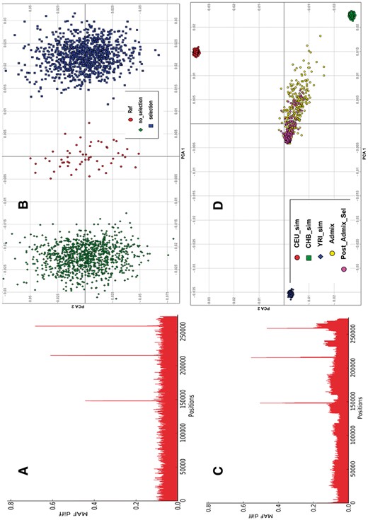
Population bottleneck and post-admixture selection. (A) Minor allele frequency difference between parental reference and simulated population bottleneck (yielding homogeneous unrelated samples, FST = 0.0021 to parental samples), indicating signal of selection at simulated variants under selection pressure. (B) PCA plot of the bottleneck simulation with and without selection and their parental CEU reference population. (C) Minor allele frequency difference between parental admixed and admixed population bottleneck, showing signal of selection at simulated variants as expected. CEU-sim, CHB-sim and YRI-sim are the simulated parental populations while Admix is the initial admixture population and Post-Admix-Sel is the post-admixture simulated population, (D) is the related PCA plot
3.3 Case-control admixture
We performed a case-control admixture simulation under the null and causal disease model, using the HapMap3 datasets. In each case we performed a three-way admixture simulation using CEU, YRI and CHB, with ancestry proportion 0.2, 0.1 and 0.7, respectively. Under the null disease model admixture simulation, we simulated a null disease model in all the pre-admixture simulations of the isolated parental populations. In the disease causal model admixture simulation, we simulated a causal model in the CHB pre-admixture simulation of the isolated population, and a null model in the CEU and YRI populations. The disease SNPs specified and the corresponding relative risk of carrying two copies and one copy of minor allele, respectively, are rs2794327 in chromosome 1 with relative risks 1.5 and 2.44, rs1177046 in chromosome 5 with relative risks 1.8 and 3.24, rs12252141 in chromosome 10 with relative risk 2.3 and 3.69, and rs3827153 in chromosome 20 with relative risks 2.0 and 3.25. In each isolated parental population simulation, we simulated 2000 cases and 2000 controls, from which we simulated 1000 admixed cases and 1000 admixed controls (FST = 0.00012 between case/control). We then performed GWAS on the simulated case-control admixed population using EMMAX (Kang et al., 2009) (from both disease null and disease causal models), as expected GWAS analysis reproduced the expected genome-wide signal on our simulated causal SNPs (Supplementary Fig. S4B and Supplementary Table S4), but no signal was detected in our null model simulation (Supplementary Fig. S4A).
3.4 Deviation in local ancestry due to selection
The current methods to infer locus-specific ancestry in multi-way admixed populations may suffer from spurious deviations in average local ancestry at some chromosomal locations of cases and controls, where the modelled ancestral population is unusually different from the true ancestral population, due to the historical action of natural selection (Chimusa et al., 2012; Pasaniuc et al., 2013). This is currently a serious weakness of admixture association (Chimusa et al., 2012; Pasaniuc et al., 2013) in most multi-way admixed populations such as the South African Coloured population (Chimusa et al., 2012, 2013). Knowing the true ancestral breakpoint, we have used a combination of three-way post-admixture with selection in Section 3.2 and case-control admixture simulation in Section 3.3, to demonstrate spurious deviations in average local ancestry (Fig. 3A–C) as selection in admixture is not modelled in most current local ancestry inference approaches. In Figure 3A–C, the true and inferred average local ancestry in cases versus controls were plotted against each other, demonstrating deviation in ancestry between cases and controls for the regions simulated under selection pressure. In addition, we assessed the ancestral breakpoints generated from the three-way admixture simulation (without selection) in Section 3.1 (Fig. 3D), and as expected, the inferred and the true local ancestry were closely related (Fig. 3D). The local ancestry inference was performed using WINPOP (Pasaniuc et al., 2009),
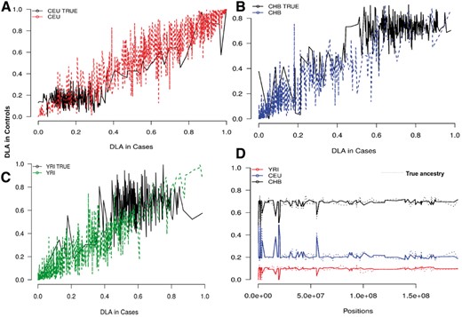
Deviations in the average local ancestry. (A–C) We plot regions of strong deviation in average local ancestry in case (x-axis) versus control (y-axis) samples of a three-way admixed population post-selection (Section 3.2). The plot shows spurious deviations in average local ancestry from the simulated region with selection pressure. (D) Evaluation of the simulated ancestral breakpoint in a normal three-way admixed population (Section 3.1)
3.5 Reproducibility of simulation processes from real datasets
To compare the simulation outcomes with real data: (i) We assessed the ability of FractalSIM to maintain the MAF, LD and haplotype structure (addition analysis in Supplementary Material S3), where we first amplified the 165 CEU samples to 1000 additional samples. Results in Figure 2A and B qualitatively illustrate that the LD patterns of the data simulated by FractalSIM are similar that of the reference panel. In Figure 2C, the allele frequencies in the parental panel with the allele frequencies of the same SNPs in the simulated data shows that allele frequencies are preserved in the simulated data. This also indicates a strong genetic correspondence between the two data. In addition, it indicates that the stochastic nature of the FractalSIM simulation is likely to conserve and mimic the genetic structure of the real data and explain any potential deviations. The PCA plot in Figure 2D shows that the simulated individuals are unrelated and closely related to parental population (FST = 2.19e−05 with an average inbreeding coefficient of 0.000223. (ii) We then mimicked the admixture scenario yielding ASW (Bryc et al., 2012) using CEU and YRI populations from 1000 Genomes data as parental populations, in a single-point scenario (the time since the admixture happened and ancestry proportion simulated are indicated in Supplementary Material S3C and Supplementary Table S7). Similar patterns of ancestry proportion between real and simulated are observed (Supplementary Fig. S6A and B and Supplementary Table S7). (iii) Finally, we mimicked the reproducibility of GWAS signal from a real case-control dataset, consisting of 873 cases and 95 controls, genotyped at 384 592 SNPs. We used the real dataset in FractalSIM to simulate a case-control homogeneous population of 1000 cases and 1000 controls (Supplementary Material S3D). FractalSIM captures LD around the simulated causal SNPs (Supplementary Table S8) from that real dataset and reproduces the GWAS signal (Fig. 4A and B). Furthermore, we observed similar patterns of heterozygosity (with an average inbreeding coefficient, F = 0.00013) in the proportion of heterozygous alleles between the real and our simulated set by plotting the observed versus expected heterozygosity (Fig. 4C). Overall FractalSIM demonstrates the ability to mimic and reproduce real genomic data. We also compare these simulation results with similar results obtained from HAPGEN2 (Supplementary Tables S9 and S10), and the results shows that FractalSIM performs better in capturing the disease signal in the real datasets, at a higher speed and requires less memory.
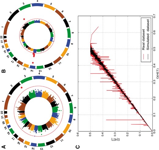
(A) GWAS analysis using a real dataset (unpublished data), (B) GWAS on simulated case-control from the real case-control and (C) proportion of observed versus expected heterozygosity in both real and simulated data. Red dots in the plots (A) and (B) indicate the significant SNPs detected (Color version of this figure is available at Bioinformatics online.)
4 Discussion and conclusion
We developed a new tool, FractalSIM, designed under the genome-wide resampling simulation approach, to mimic various population genetics models. The tool offers users the option to simulate various scenarios of population bottlenecks, complex admixture, selection and disease models. The user interacts with the tool through a parameters file, where they can define the desired simulation and specify the related simulation parameters. FractalSIM integrates several population genetics models, and shows promise for the evaluation of current and future analytical genomics methods. The current version of FractalSIM has some limitations; including (i) It is limited to only simulated bi-allelic SNPS of minor allele frequency > 0.05, (ii) although its computational cost is reasonable (Supplementary Table S8), this currently increases with sample size and number of variants to be simulated. FractalSIM can be run on cluster machines with the option to parallelize jobs to address the computational cost. Although subsequent versions will be developed, the current version is still useful to the genomics research community and has two advantages over existing tools: (i) it integrates several genetics simulation models into one framework and (ii) it has the ability to simulate genome-wide data. Additional simulation models, such as gene–environment, gene–gene interaction in disease models and further nuances of whole genome data such as genotype likelihood, error rate and depth, will be integrated in future versions of the tool.
Acknowledgements
We thank all study participants for the dataset used. Computations were performed using facilities provided by the University of Cape Town’s ICTS High Performance Computing team (http://hpc.uct.ac.za) and the Centre for high performance computing (CHPC, South africa).
Funding
Some of the authors are funded in part by the National Institutes of Health Common Fund under grant number U41HG006941, the Government of Canada via the International Development Research Centre (IDRC) through the African Institute for Mathematical Sciences, University of Cape Town, the German Academic Exchange Service (DAAD) and the Organization for Women in Science for the Developing World (OWSD) scholarships.
Conflict of Interest: none declared.
References

