


Abstract
Despite recent advances in algorithms design to characterize structural variation using high-throughput short read sequencing (HTS) data, characterization of novel sequence insertions longer than the average read length remains a challenging task. This is mainly due to both computational difficulties and the complexities imposed by genomic repeats in generating reliable assemblies to accurately detect both the sequence content and the exact location of such insertions. Additionally, de novo genome assembly algorithms typically require a very high depth of coverage, which may be a limiting factor for most genome studies. Therefore, characterization of novel sequence insertions is not a routine part of most sequencing projects.
There are only a handful of algorithms that are specifically developed for novel sequence insertion discovery that can bypass the need for the whole genome de novo assembly. Still, most such algorithms rely on high depth of coverage, and to our knowledge there is only one method (PopIns) that can use multi-sample data to “collectively” obtain a very high coverage dataset to accurately find insertions common in a given population.
Here, we present Pamir, a new algorithm to efficiently and accurately discover and genotype novel sequence insertions using either single or multiple genome sequencing datasets. Pamir is able to detect breakpoint locations of the insertions and calculate their zygosity (i.e. heterozygous versus homozygous) by analyzing multiple sequence signatures, matching one-end-anchored sequences to small-scale de novo assemblies of unmapped reads, and conducting strand-aware local assembly. We test the efficacy of Pamir on both simulated and real data, and demonstrate its potential use in accurate and routine identification of novel sequence insertions in genome projects.
Pamir is available at https://github.com/vpc-ccg/pamir.
Supplementary data are available at Bioinformatics online.
1 Introduction
Genomic structural variations (SVs) are broadly defined as alterations that affect more than 50 base pairs (bp) of DNA (Alkan et al., 2011), and they have major impact on both evolution and human disease (Alkan et al., 2011; Sharp et al., 2006). Such alterations may be in various forms including deletions, insertions, inversions, duplications, and retrotranspositions (Alkan et al., 2011). Thanks to the wide availability and cost efficiency of high throughput sequencing (HTS), we now have the ability to characterize SVs in the genomes of many individuals, as exemplified by large-scale projects such as the 1000 Genomes Project (Mills et al., 2011; The 1000 Genomes Project Consortium, 2015). Accurate characterization of SVs required the development of many novel algorithms (Alkan et al., 2011; Medvedev et al., 2009) that are benchmarked within the 1000 Genomes and the Genome in a Bottle (Zook et al., 2014) projects.
Novel sequence insertions, or alternatively, “deletions from the reference”, are genomic segments that are not represented in the reference genome assembly (Kidd et al., 2010a). Similar to “deletions from the sequenced sample”, they may harbor sequences of functional importance such as coding exons or regulatory elements (Kidd et al., 2010a), which underline the importance of their accurate characterization. The non-reference sequences identified in various genome studies are thus “added” to the reference genome as additional sequence. However, due to the complexity of these new sequences and their polymorphism in different populations, there is now a push towards building graph-based representations (Church et al., 2015; The Computational Pan-Genomics Consortium, 2017).
Although several forms of SVs such as deletions, tandem duplications and mobile element insertions are investigated to a certain extent (Alkan et al., 2011; Chaisson et al., 2015a,b), characterization of novel sequence insertions longer than read lengths is still lagging. This is mainly because long sequence insertions can be discovered only through sequence assembly, which is computationally challenging and may lead to incorrect or fragmented sequence reconstructions due to common repeats that may lie within or close to such insertions (Hajirasouliha et al., 2010; Kidd et al., 2010a). Cortex (Iqbal et al., 2012) aims to improve the accuracy in complex regions by using colored de Bruijn graphs, but a recent study found that it has high computational requirements (Kehr et al., 2015).
Aside from computationally intensive assembly-based algorithms, only a handful of mapping and local assembly based methods for novel sequence insertion discovery are currently available. The first of such algorithms is NovelSeq (Hajirasouliha et al., 2010) that we have previously developed to find insertions >200 bp using paired-end whole-genome Illumina sequence data. Briefly, NovelSeq identifies one-end anchored reads (OEA), where one end of a pair maps to the reference and the other remains unmapped, and calculates the best match between local assembly of OEA reads and de novo assembly of orphan (both ends unmapped) reads to identify both the content and the approximate location of the insertion. However, NovelSeq was designed to analyze one genome at very high sequence coverage. It could find insertions of length up to a couple of kilobase pairs, but it does not provide the exact content of the insertion, the exact breakpoint location and the genotyping information. MindTheGap (Rizk et al., 2014) was developed for finding insertion breakpoints and their sequences in a single sequenced genome based on an assembly-first strategy. BASIL & ANISE (Holtgrewe et al., 2015) are also designed for detecting novel sequence insertions where BASIL detects the breakpoints by clustering one-end anchored reads and ANISE assembles the novel insertions with an overlap-layout-consensus graph based assembler.
A more recent algorithm, PopIns (Kehr et al., 2015) follows a similar approach and also incorporates the split-read sequence signature (Alkan et al., 2011) to discover and then genotype common sequence insertions within a large cohort of samples. Using “soft-clipped” reads, another algorithm Swan (Xia et al., 2016) can only find breakpoints of long insertions without providing its content.
In this paper, we present Pamir, a new tool to provide exact breakpoint positions, sequence contents, and genotypes of novel sequence insertions either in single or multiple genomes sequenced with the Illumina technology. We show that, when a single genome is used, it outperforms MindTheGap (Rizk et al., 2014), BASIL & ANISE (Holtgrewe et al., 2015), and PopIns (Kehr et al., 2015). Additionally, using simulated low coverage data (5 samples at 10X coverage each) we demonstrate that Pamir has better precision and recall rates than PopIns, which is the only other insertion characterization tool that can use multiple genomes.
2 Materials and methods
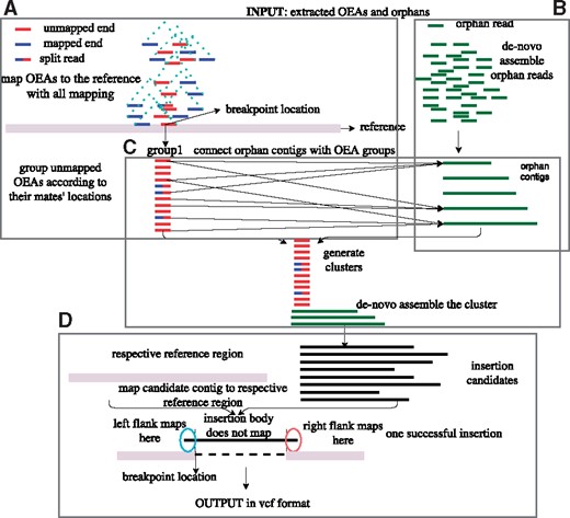
We developed Pamir to characterize novel sequence insertions using paired-end whole genome sequencing (WGS) data generated by the Illumina platform. Pamir is based on the observation that structural events such as “novel sequence insertion” leave a group of one-end anchors, i.e. one-end is mapped while the other is unmapped, around their breakpoint location when aligning the donor sequences to the reference genome (Hajirasouliha et al., 2010; Kidd et al., 2010a,b). Furthermore, the insertions longer than the paired-end fragment size will leave another group of reads known as orphan reads, i.e. read pairs where none of the ends can be mapped to the reference. Figure 1 depicts the mapping information in the vicinity of the hypothetical novel insertion. Pamir uses both types of reads to characterize the novel sequence contents and their insertion breakpoints. First, it starts with generating a de novo assembly of the orphan reads to obtain orphan contigs. Next, Pamir clusters the OEA read pairs based on their mapping locations on the reference genome. It then remaps the OEA reads to orphan contigs to match the orphan contigs with OEA clusters. Finally, it outputs the putative novel insertion by assembling the updated cluster and re-aligning the generated contig to the respective reference region (Fig. 2). In this section, we provide a detailed description of the Pamir algorithm.
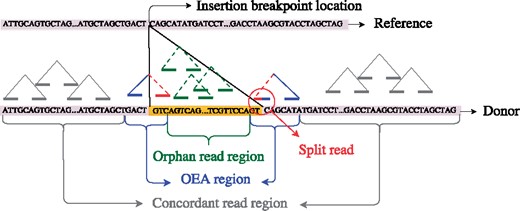
Classification of donor sequence regions in terms of read mappings. Concordant read: both ends map in correct orientation and within expected insert size. OEA read: one-end anchored, only one end maps to the reference. Split read is an OEA read whose unmapped end crosses the breakpoint and generates split mapping. Orphan read: none of the ends map to the reference
General overview of Pamir
Pamir versus NovelSeq. While they both are based on similar observations, Pamir significantly improves accuracy, performance, and usability of NovelSeq. For a candidate insertion breakpoint location, NovelSeq first assembles two OEA clusters on its upstream (OEA+) and downstream side (OEA-), and then matches these two OEA contigs with orphan contigs. Rather than providing precise breakpoints and insertion content, NovelSeq reports a range of breakpoint locations based on associations between OEA contigs and orphan contigs. On the other hand, Pamir collects nearby OEAs to build a cluster, and includes all relavant orphan contigs to this cluster based on the association obtained from mapping OEA reads to orphan contigs. It then assembles each cluster and obtains the insertion content through aligning the contig to the respective reference region. Combined with the post-analysis steps, Pamir provides the breakpoint locations at single-nucleotide resolution, exact insertion content, and genotype information, which are all missing in NovelSeq.
2.1 Pre-processing
Pamir accepts both raw reads (in FASTQ format) or aligned reads (in SAM/BAM files) as input. If raw reads are provided, Pamir first maps them to the reference genome using mrsFAST-Ultra (Hach et al., 2010, 2014) in best mapping mode. Pamir skips the mapping step if the read alignment is provided, i.e. BAM file. Next, Pamir extracts OEA and orphan reads using the alignment results. Pamir then remaps the OEA reads using mrsFAST-Ultra in multi-mapping mode since the breakpoints of a sequence insertion may lie within repeats, which causes mapping ambiguity (Bailey et al., 2001; Firtina and Alkan, 2016) (Fig. 2A). Using multi-mapping locations may introduce false positives in repeat regions, which we eliminate in a post-processing step. Pamir assembles the orphan reads using Velvet (Zerbino and Birney, 2008) with the k-mer length set to 31 bp, although any other assembler may also be used for this step (Fig. 2B). After the assembly, we subject the contigs to a contaminant filter by querying the nt/nr database, and we remove those contigs that map to vector and/or bacterial sequences and other known contaminants. We then map the unmapped end of OEA read pairs to the orphan contigs using mrsFAST-Ultra in the multi-mapping mode to match the OEAs to the corresponding orphan contigs. In this way, the OEA-to-orphan remapping stage allows an OEA to be aligned to more than one orphan contig (Fig. 2C). To avoid missing any associations between split reads (Fig. 1) and orphan contigs, we also split the unmapped OEAs from the previous stage into a half, i.e. balanced splits, and remap them to the orphan contigs.
In summary, the pre-processing step generates four types of information required to discover a novel sequence insertion event: (i) the mapping information of the OEA mapped reads; (ii) unmapped OEA sequences; (iii) orphan contigs; and (iv) pairwise association between unmapped OEA reads and orphan contigs.
2.2 Cluster formation
Pamir clusters OEAs based on the mapping locations of their mapped end to detect potential insertion breakpoints. It then employs an iterative greedy strategy, which anchors the first cluster with the leftmost mapping locus x of an OEA on the genome. Next, it extends the cluster to include any other OEA mappings overlapping with the interval where L is the fragment size (Let L be the fragment size of paired-end reads which can be estimated from concordant mappings. For an insertion in breakpoint p, most of its OEA anchors should be mapped within , which spans a 2 interval on the reference genome). Once all such OEA mappings are added to the existing cluster, the iterative strategy then greedily anchors the next cluster with the first OEA mapping that is not included in the previous cluster. Note that in this strategy each OEA mapping can only be part of a single cluster. However, a single read pair may generate multiple OEA mappings (and thus belong to multiple OEA clusters) due to the use of multi-mapping strategy.
After the first clustering pass is completed, Pamir adds the unmapped OEA mates of the reads and their associated orphan contigs into each cluster (Fig. 2C). To find the associated orphan contigs, the “OEA-to-orphan contig” mapping information generated in the pre-processing step is used. A contig is added to a cluster if (i) the cluster contains OEAs that map to the both ends of the orphan contig; or (ii) at least 30% of the OEAs in the cluster map only to either end of the contig. We allow the second condition to avoid missing any partially assembled orphan contigs.
In summary, each cluster generated in this step contains the following information: (i) the number of the OEA reads and their associated contigs; (ii) the leftmost OEA mapping location; (iii) the rightmost OEA mapping location; (iv) unmapped OEA read information (see below); and (v) contigs associated with unmapped OEA reads. For each unmapped end of an OEA read pair, the following information is kept in the cluster: (i) read name; (ii) strand (based on its corresponding mapped mate); and (iii) read sequence.
2.3 Insertion discovery
2.3.1 Candidate insertion contig assembly
Pamir generates a new assembly for each cluster to compute the putative insertion that consists of both left and right flanking regions that overlap with the reference genome and its main body which constitutes the insertion (Fig. 2C). The resulting cluster-aware assembly represents a potential novel insertion sequence.
We assemble the reads and contigs in each cluster using an efficient in-house overlap-layout-consensus (OLC) assembler. We found most of the available off-the-shelf assemblers to be too slow for this task, especially because the total number of clusters is measured in millions. Additionally, existing tools cannot be modified to consider strand information that can be inferred from the mapping information while our in-house assembler is strand-specific. Furthermore, use of naïve greedy strategy for assembly is not suitable for our goal because such method cannot obtain optimal contigs necessary for accurate insertion detection.
The objective of the in-house assembler is to construct a contig that maximizes the total sum of overlaps between the reads. This problem can be optimally solved by modeling it as an instance of maximum weighted path problem in a directed graph G(V, E) as follows. Let each vertex v represent a read in the cluster. Two vertices m and v are connected with a directed edge of weight if the maximum prefix-suffix overlap between the reads represented by those vertices is of length . We can optimally calculate the maximum weighted path via a dynamic programming formulation as follows.
However, both topological sorting and Equation (1) require acyclic G, which might not be always true, especially if the target region contains some repeat. In that case, maximum weighted path problem is NP-hard, which can be easily shown by reducing the longest path problem in a graph to the maximum weighted path problem. If cycles are present, we remove any cycle from G in a greedy fashion by iteratively removing cycle edges whose endpoint is the vertex with the smallest indegree in G in order to provide a feasible assembly. Because the size of each cluster is small, and because the repeats are not often present in G, such cyclic graphs are not common. Thus, in the majority of the cases, our assembler is guaranteed to produce an optimal assembly for a given cluster.
2.3.2 Breakpoint and content detection
The cluster assembly provides the sequence content. The insertion breakpoint can be inferred using the provided assembled contigs, the leftmost and the rightmost mapping locations kept for each cluster. Thus, to characterize the exact insertion breakpoint, we align the assembled contigs to the reference in the vicinity of each cluster using a modified variant of Smith-Waterman (Smith and Waterman, 1981) algorithm where the assembled contig is fully aligned to a substring of the genomic sequence, i.e. global to local alignment. We only consider those candidate insertions that align to the reference by at least 6bp at both sides. We finally return the sequence between these two flanking sequences as the novel insertion and the end of the left-mapping flank as the exact breakpoint location (Fig. 2D).
2.4 Post-processing and genotyping
2.4.1 False positive removal
To refine our candidate list and eliminate false positives, for a dataset with fragment size L, we construct a temporary reference segment by concatenating three sequences: (i) L bp upstream of the breakpoint from the reference; (ii) the obtained insertion sequence from the previous step; and (iii) L bp downstream of the breakpoint from the reference. We then map all OEAs and orphan reads to this temporary reference and we report the insertion if for each breakpoint, there exists a concordant mapping in which only one mate overlaps the insertion sequence and the other mate is in the flanking region. With this method, we guarantee that both breakpoints are covered by supporting reads, which are signatures of an insertion. A false positive case will miss these reads and will be eliminated.
2.4.2 Mapping ambiguity resolution
There might be still some reads which map to multiple novel insertions. We assign each such read to the insertion with the highest support via set-cover algorithm, where the set of reads represents the universe, and where clusters represent the sets. By selecting the minimal number of sets which describe all of the available reads, we eliminate low-support insertions and ensure that each read belongs to only one insertion event. Because the set cover is an NP-hard problem, we use a fast greedy strategy to calculate the minimal set of events that covers all reads (Johnson, 1974).
2.4.3 Genotyping
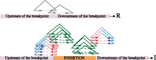
Genotyping novel sequence insertions with Pamir. Here we show an example for calculating r, i and x based on the Figure: r = 2 (the # of mappings passing through the breakpoint on R); il = 9 (the # of mappings passing through the left breakpoint on I); ir = 7 (the # of mappings passing through the right breakpoint on I); i = (il+ir)/2 = 8; x = (i-r)/(i + r) = 0.6
2.5 Discovery with pooled data
Pamir supports population-scale insertion discovery by first detecting insertions in pooled samples, and then genotyping all events in each sample. In other words, Pamir extracts OEAs and orphans from all samples to construct one OEA dataset and one orphan dataset. It then analyzes the combined dataset to detect the list of potential insertions for the whole population. After obtaining the initial list of potential insertions, Pamir genotypes each insertion for each sample using the reads from that specific dataset, as explained in Section 2.4.
3 Results
We performed four sets of experiments to evaluate our method: two experiments with simulated data, and two experiments using real data.
In simulation experiments, we inserted 350 new sequences into chromosome 21 of the GRCh37 reference in 7 different size ranges (10–100 bp, 100–200 bp, 200–500 bp, 500–1K bp, 1K–2K bp, 2K–5K bp, 5K–10K bp) with each range containing 50 insertions. We used randomly selected segments from the Methylobacterium reference genome for this purpose, which are guaranteed to be missing in the human genome reference. Next we generated 6 high coverage WGS datasets using the ART read simulator (Huang et al., 2012) to test Pamir under different conditions:
error-free reads generated as (a) 2x100bp Illumina HiSeq 2000, (b) 2x100bp Illumina HiSeq 2500, and (c) 2x150bp Illumina HiSeq 2500;
noisy reads, i.e. introduced small variants as SNPs and indels and sequencing errors, generated as (a) 2x100bp Illumina HiSeq 2000, (b) 2x100bp Illumina HiSeq 2500, and (c) 2x150bp Illumina HiSeq 2500.
All 6 high coverage simulated datasets were created at 30x sequence coverage using default parameters of ART that are set for each sequencing machine’s error model.
We also evaluated the efficacy of Pamir on low-coverage multi-sample data. For this purpose, we simulated 5 2x100bp WGS datasets at 10x sequence coverage using ART’s default parameters for noisy Illumina HiSeq 2500 sequencer. Each of the 5 datasets is sampled from a different simulated genome: the first genome includes all 350 novel insertions, and the remaining 4 each includes 280 randomly selected insertions. In all single-sample simulation experiments we compared Pamir with MindTheGap, BASIL & ANISE, and PopIns using their default parameters. In multi-sample datasets, we compared Pamir with PopIns (the only tool before Pamir capable of finding insertions in multi-sample data), using default parameters of PopIns.
We tested Pamir on real datasets in two experiments. First, we applied Pamir on a high coverage WGS dataset generated from a single haploid sample (CHM1) (Chaisson et al., 2015b) and compared our results with novel insertions found in the same genome with the SMRT-SV algorithm that uses long read, i.e. Pacific Biosciences, sequencing technology. Finally, we evaluated Pamir ’s performance in multi-sample insertion discovery and genotyping using 10 low-coverage WGS datasets generated as part of the 1000 Genomes Project (The 1000 Genomes Project Consortium, 2015).
3.1 Simulations
3.1.1 High coverage single sample
We compared all tools in terms of precision (, where TP is number of True Positives and FP is number of False Positives) and recall (, where TP is number of True Positives and FN is number of False Negatives). We summarize the results of our simulation experiment in Table 1. Briefly, Pamir outperforms BASIL & ANISE, MindTheGap and PopIns in all simulation experiments in terms of recall. In terms of precision, Pamir outperforms PopIns and BASIL & ANISE; and has better or equal precision to MindTheGap. Here we consider a predicted insertion to be correct only if the breakpoint matches that of the simulated insertion. Note that if we also require the lengths of the predicted insertions to be the same with the simulation, Pamir has the best precision and recall among the tools we tested (Supplementary Table S10 and Supplementary Fig. S1). We present range specific precision recall rates of all tools for error-free Illumina HiSeq2000-100bp data in Table 2. A detailed version of this table can be found in Supplementary Table S1.
Precision and recall of Pamir, PopIns, MindTheGap and BASIL & ANISE on simulated 30x datasets generated for different sequencing platforms with varying read lengths
| Error free | Noisy | |||||||||||
|---|---|---|---|---|---|---|---|---|---|---|---|---|
| HiSeq2500-100 bp | HiSeq2500-150 bp | HiSeq2000-100 bp | HiSeq2500-100 bp | HiSeq2500-150 bp | HiSeq2000-100 bp | |||||||
| Pa | Rb | Pa | Rb | Pa | Rb | Pa | Rb | Pa | Rb | Pa | Rb | |
| Pamir | 1.000 | 0.954 | 1.000 | 0.960 | 1.000 | 0.951 | 1.000 | 0.926 | 1.000 | 0.943 | 1.000 | 0.826 |
| PopIns | 0.973 | 0.814 | 0.958 | 0.726 | 0.972 | 0.823 | 0.969 | 0.800 | 0.968 | 0.789 | 0.938 | 0.709 |
| MindTheGap | 1.000 | 0.900 | 1.000 | 0.900 | 1.000 | 0.900 | 1.000 | 0.900 | 0.965 | 0.897 | 0.905 | 0.811 |
| BASIL & ANISE | 0.989 | 0.757 | 0.989 | 0.763 | 0.989 | 0.763 | 0.989 | 0.757 | 0.989 | 0.754 | 0.974 | 0.743 |
Best results are marked with bold typeface.
Precision.
Recall.
Precision and recall rates of perfect Illumina HiSeq2000-100 bp simulation data with respect to different ranges of insertion sizes where each range contains 50 insertions
| Insertion | Pamir | PopIns | MindTheGap | BASIL & ANISE | ||||
|---|---|---|---|---|---|---|---|---|
| Length (bp) | Ra | Pb | Ra | Pb | Ra | Pb | Ra | Pb |
| 10–100 | 1.00 | 1.00 | 0.10 | 1.00 | 0.88 | 1.00 | 0.00 | 1.00 |
| 100–200 | 1.00 | 1.00 | 0.82 | 0.98 | 0.92 | 1.00 | 0.60 | 1.00 |
| 200–500 | 1.00 | 1.00 | 0.84 | 0.95 | 0.92 | 1.00 | 1.00 | 1.00 |
| 500–1K | 0.98 | 1.00 | 1.00 | 0.98 | 0.88 | 1.00 | 0.98 | 1.00 |
| 1K–2K | 0.96 | 1.00 | 1.00 | 0.94 | 0.92 | 1.00 | 1.00 | 0.98 |
| 2K–5K | 0.92 | 1.00 | 1.00 | 0.93 | 0.84 | 1.00 | 0.98 | 1.00 |
| 5K–10K | 0.80 | 1.00 | 1.00 | 0.93 | 0.94 | 1.00 | 0.98 | 1.00 |
| Total | 0.95 | 1.00 | 0.82 | 0.97 | 0.90 | 1.00 | 0.76 | 0.99 |
Best results for total are highlighted in boldface.
R: Recall.
P: Precision.
3.1.2 Low coverage multiple samples
Next, we tested the prediction performance of Pamir when multiple genomes with low coverage data are available. In this experiment we compared Pamir only with PopIns, as it is the only other multi-sample novel sequence insertion discovery tool. To evaluate the importance of multiple samples, we tested the same five genomes simulated at 10x sequence coverage both separately and collectively (Table 3). We found that Pamir ’s precision was substantially higher than that of PopIns when each sample is processed separately, and use of multiple genomes resulted in higher recall rates for both tools.
Precision and recall rates of 5 simulated samples (noisy HiSeq2500 2*100 bp 10x)
| Pooled | Individual | |||||||||||
|---|---|---|---|---|---|---|---|---|---|---|---|---|
| Samples | All | S1 | S2 | S3 | S4 | S5 | ||||||
| # of Insertions | 350 | 350 | 280 | 280 | 280 | 280 | ||||||
| Pa | Rb | Pa | Rb | Pa | Rb | Pa | Rb | Pa | Rb | Pa | Rb | |
| Pamir | 1.000 | 0.911 | 1.000 | 0.726 | 1.000 | 0.711 | 1.000 | 0.704 | 1.000 | 0.714 | 1.000 | 0.714 |
| PopIns | 0.977 | 0.811 | 0.575 | 0.657 | 0.591 | 0.675 | 0.575 | 0.657 | 0.574 | 0.646 | 0.603 | 0.668 |
Best results are marked with bold typeface.
Precision.
Recall.
Precision and recall rates of both individual and pooled calls of five low coverage samples. The paired-end reads (2*100 bp) are generated using Illumina HiSeq2500 error model. We have simulated 350 insertions in this dataset: S1 have all insertions, and genomes of the other four individuals contains 280 events. The column All shows performances of Pamir and PopIns based on pooling simulation reads, and each column Si represents single sample detection results for i-th individual.
We also predicted genotypes on all five samples using Pamir (Table 4). Here we first characterized insertions using all five samples simultaneously as described above, and then calculated genotypes for each predicted insertion in all samples separately. We observed no incorrect heterozygous versus homozygous genotyping results for any insertions, except 5 calls in 3 samples are identified as heterozygous although they were homozygously inserted. All 5 insertions map to common repeats, i.e. LINE elements.
Evaluation of predicted genotypes using 5 simulated genomes
| Samples | S1 | S2 | S3 | S4 | S5 | |||||
|---|---|---|---|---|---|---|---|---|---|---|
| # of Insertions | 350 | 280 | 280 | 280 | 280 | |||||
| # of Insertions not in the sample | 0 | 70 | 70 | 70 | 70 | |||||
| Pamir | PopIns | Pamir | PopIns | Pamir | PopIns | Pamir | PopIns | Pamir | PopIns | |
| Correct (INS) | 317 | 284 | 253 | 210 | 252 | 214 | 253 | 225 | 259 | 227 |
| Correct (REF) | – | – | 66 | 54 | 66 | 56 | 64 | 59 | 60 | 57 |
| Incorrect zygosity | 2 | 0 | 0 | 0 | 1 | 0 | 2 | 0 | 0 | 0 |
| No call (INS) | 31 | 66 | 27 | 50 | 27 | 52 | 25 | 55 | 21 | 53 |
| No call (REF) | – | – | 4 | 16 | 4 | 14 | 6 | 11 | 10 | 13 |
Best results are marked with bold typeface.
Evaluation of genotyping results for the same five samples as in Table 3, based on pooling simulated reads. The paired-end reads (2*100 bp) are generated using Illumina HiSeq2500 error model. We have simulated 350 insertions in this dataset: S1 have all insertions, and genomes of the other four individuals contains 280 events. Correct (INS) lists the number of insertions that are correctly genotyped. Correct (REF) shows the number of detections discarded after genotyping, which are not actual insertions in an individual but falsely predicted based on pooling reads. Incorrect zygosity provides the number of insertions incorrectly genotyped as heterozygous; only 5 calls were identified as heterozygous in S1, S3 and S4 although they were homozygously inserted. All insertions map to common repeats. The No call (INS) row shows the number of insertions missed in the pooled run for each sample, i.e. false negatives. No call (REF) provides the number of insertions missed in the pooled run but the insertion was not inserted into this sample.
3.2 Real data
3.2.1 High coverage sequencing of CHM1
Our tests using real data also included two types of datasets: i) high coverage single sample WGS, and ii) low coverage multiple sample WGS. First, we evaluated Pamir using WGS data at 40x coverage generated from a haploid cell line with the Illumina technology (CHM1, SRA ID: SRX652547) (Chaisson et al., 2015b). We have identified a total of 22,676 insertions that corresponds to 593.5 Kb in total, of which, 2,444 were >50bp (348 Kb total) (Table 5). Chaisson et al. (2015) also generated de novo assembly of the same genome using a long read sequencing technology (Pacific Biosciences) from the same cell line, and predicted insertions with the SMRT-SV algorithm using this dataset (Chaisson et al., 2015b). Here we used an updated call set (bp) mapped to human GRCh38 (Huddleston et al., 2016) for comparisons. Pamir showed low recall rates when compared to the long read-based SMRT-SV results (Chaisson et al., 2015b). We could identify only 488 of the 12,998 insertions detected by SMRT-SV when we consider only nearby matches (less than 10bp distance) in breakpoint predictions. One of the reasons for such discrepancy is the fact that more than half of PacBio-predicted insertions are located within various repeat regions (Table 6), and short-length Illumina reads are not sufficient to properly assemble such regions. The same effect was also observed in the original publication (Chaisson et al., 2015b), where only a handful of insertions were also identified in another assembly of the same genome that was constructed with a reference-guided methodology using both Illumina WGS and bacterial artificial chromosome datasets (Steinberg et al., 2014). We observed that approximately 45% of the insertions characterized by SMRT-SV are contain either very low () or high () GC%, which are known to be problematic to sequence using the Illumina platform (Benjamini and Speed, 2012; Ross et al., 2013). Additionally, we found that 14,121 out of our 22,676 predicted insertions were reported in dbSNP version 147 (Within 10 bp breakpoint resolution.).
Summary of insertions predicted in CHM1
| All | 50bp | > 50bp | |
|---|---|---|---|
| Number of insertions | 22,676 | 20,232 | 2,444 |
| Minimum length | 5 | 5 | 51 |
| Maximum length | 4,135 | 50 | 4,135 |
| Average length | 26.20 | 12.12 | 142.51 |
| All | 50bp | > 50bp | |
|---|---|---|---|
| Number of insertions | 22,676 | 20,232 | 2,444 |
| Minimum length | 5 | 5 | 51 |
| Maximum length | 4,135 | 50 | 4,135 |
| Average length | 26.20 | 12.12 | 142.51 |
Comparison of insertions in CHM1 by SMRT-SV using PacBio reads versus Pamir and PopIns using Illumina reads allowing 10bp breakpoint resolution
| PacBio | Illumina | ||||
|---|---|---|---|---|---|
| SMRT-SV | Pamir | PopIns | |||
| Insertion Length | Prediction | Prediction | Shared with SMRT-SV | Prediction | Shared with SMRT-SV |
| 1–50 bp | 187a (60%, 57%) | 20,232 (56%, 38%) | 27 (63%, 14%) | 21 (71%, 24%) | 0 |
| 50–100 bp | 4,384 (54%, 53%) | 1,273 (70%, 18%) | 205 (52%, 14%) | 246 (73%, 4%) | 17 (70%, 0%) |
| 100–200 bp | 2,959 (54%, 50%) | 815 (75%, 13%) | 125 (58%, 13%) | 793 (66%, 4%) | 120 (62%, 1%) |
| 200–500 bp | 3,123 (55%, 37%) | 291 (74%, 7%) | 97 (61%, 1%) | 1,074 (65%, 3%) | 141 (58%, 1%) |
| >500 bp | 2,345 (60%, 32%) | 65 (63%, 3%) | 34 (50%, 3%) | 1,286 (59%, 3%) | 207 (51%, 1%) |
| All | 12,998 (55%, 45%) | 22,676 (58%, 36%) | 488 (56%, 10%) | 3,420 (58%, 3%) | 485 (56%, 1%) |
For each category, we report (i) the percentile of the calls that fall into repeat regions compared to repeat masker file, and (ii) the percentile of the calls with biased GC ratios (20% or 60%) in the form (% of repeat regions, % of biased GC ratios) in the parentheses.
All events reported have a length of 50bp. Note that the comparisons are based only on breakpoint positions without consideration about contents of insertions. If we simultaneously consider insertion lengths and contents, most of PopIns predictions will be filtered out as shown in Supplementary Tables S5 and S6. It is worth mentioning that Pamir can call most of the predictions as PopIns. However, it filters most of them because of the stringent rules.
To test whether the insertions we predicted in CHM1 were also previously discovered in other studies, we mapped the longer insertions (>50 bp) with spanning regions around the breakpoint on the reference (GRCh37) to the latest version of the reference (GRCh38) using BLAST (Altschul et al., 1990). Note that our predictions were based on the GRCh37 version. In this experiment we required only highly identical (98%) hits that covered at least 98% of the predicted insertion. We repeated the same remapping experiment to both the long read-based assembly (Chaisson et al., 2015b) and the alternative reference-guided assembly of the same genome (Steinberg et al., 2014). Finally, we also mapped the same sequences to the nt/nr database to detect whether the sequences were also contained within other WGS studies, in particular, fosmid end-sequence data (Kidd et al., 2008). In summary, out of 2,444 (> 50 bp) insertions we predicted, 1,446 are not found in any database, of which 1,212 mapped to common repeats (Table 7). We performed the same experiment using PopIns (Table 7). 1,014 out of 3,399 PopIns calls are not found in any database, of which 388 mapped to common repeats. 56% of PopIns calls map to long insert clones, but only a handful were included in the latest version of the human genome reference, and assemblies of the same DNA resource.
Hierarchical non-redundant analysis of predicted CHM1 insertions with Pamir and PopIns with respect to other datasets
| Pamir | PopIns | |||||||
|---|---|---|---|---|---|---|---|---|
| 50 - 200 bp | 200 - 500 bp | >500 bp | Total | 50 - 200 bp | 200 - 500 bp | >500 bp | Total | |
| # of insertions | 2,088 | 291 | 65 | 2,444 | 1,038 | 1,075 | 1,286 | 3,399 |
| In GRCh38 | 17 | 1 | 1 | 19 | 0 | 1 | 1 | 2 |
| In CHM1_1.1 (Steinberg et al., 2014) | 251 | 54 | 2 | 307 | 15 | 8 | 1 | 24 |
| In CHM1 PacBio (Chaisson et al., 2015b) | 213 | 13 | 23 | 249 | 5 | 2 | 12 | 19 |
| In SMRT-SV (Huddleston et al., 2016) | 73 | 47 | 11 | 131 | 118 | 132 | 193 | 443 |
| In long insert clonesa (Kidd et al., 2008) | 212 | 21 | 1 | 234 | 565 | 627 | 705 | 1,897 |
| In repeat regions | 1,065 | 126 | 21 | 1,212 | 221 | 191 | 214 | 626 |
| Remainder | 257 | 29 | 6 | 292 | 114 | 114 | 160 | 388 |
Here we provide a hierarchical non-redundant breakdown of comparison of insertions we predicted in the CHM1 genome with Pamir and PopIns. We compare the predictions in the following order: the GRCh38 assembly, then remaining to the reference-guided CHM1_1.1 assembly, the Pacific Biosciences (PacBio) assembly, SMRT-SV call set, long insert clones and those that are in repeat regions.
Long insert clones include both fosmid clones and bacterial artificial chromosomes (BAC). Since we apply more stringent rules to filter false positives in Pamir, many of our discarded calls are still kept by PopIns. This will affect recall rate of Pamir, especially for longer insertions whose orphan contigs are difficult to be assembled.
3.2.2 Low coverage genomes from the 1000 genomes project
Finally, we tested Pamir using low coverage WGS datasets generated from 10 samples as part of the 1000 Genomes Project (The 1000 Genomes Project Consortium, 2015) (Table 8). We found 39,554 insertions when we pooled all 10 genomes, 13,255 of them were reported in 1000 Genomes project, and another group of 11,019 insertions was seen in dbSNP version 147 (Considering 10 bp breakpoint resolution.). We then genotyped for each sample (Table 9).
Summary of novel sequences found in 10 low coverage WGS datasets from the 1000 Genomes Project
| Total | > 50bp | |
|---|---|---|
| Number of insertions | 49,473 | 6,846 |
| Minimum length | 5 | 51 |
| Maximum length | 1,928 | 1,928 |
| Average length | 28.872 | 128.085 |
| In 1000 Genomes Project | 14,837 | 425 |
| In dbSNP version 147* | 14,409 | 2,027 |
| Total | > 50bp | |
|---|---|---|
| Number of insertions | 49,473 | 6,846 |
| Minimum length | 5 | 51 |
| Maximum length | 1,928 | 1,928 |
| Average length | 28.872 | 128.085 |
| In 1000 Genomes Project | 14,837 | 425 |
| In dbSNP version 147* | 14,409 | 2,027 |
*We intersected with dbSNP after removing those insertions that are found in the 1000 Genomes Project.
Genotyping results for the novel sequences found in the 1000 Genomes Project datasets
| Homozygous | Heterozygous | Total insertion length (bp) | |
|---|---|---|---|
| NA06985 | 22,971 | 10,246 | 941,868 |
| NA07357 | 22,582 | 10,158 | 921,225 |
| NA10851 | 23,274 | 9,465 | 930,766 |
| NA11840 | 20,973 | 12,745 | 959,017 |
| NA11918 | 22,610 | 9,994 | 953,968 |
| NA11933 | 21,049 | 11,092 | 936,615 |
| NA12004 | 19,024 | 12,650 | 928,371 |
| NA12044 | 18,753 | 13,002 | 919,212 |
| NA12234 | 20,841 | 10,804 | 916,251 |
| NA12286 | 19,027 | 12,622 | 922,799 |
To test whether the insertions we predicted in these 10 samples were also previously discovered in other studies, we mapped the longer insertions (>50 bp) to the latest version of the reference (GRCh38) using BLAST (Altschul et al., 1990). We also mapped the same sequences to the nt/nr database (Table 10).
(Pamir & PopIns) Analysis of insertions found in low-coverage samples with respect to other datasets
| Pamir | PopIns | |||||||
|---|---|---|---|---|---|---|---|---|
| 50–200 bp | 200–500 bp | >500 bp | Total | 50–200 bp | 200–500 bp | >500 bp | Total | |
| # of insertions | 6,050 | 667 | 129 | 6,846 | 5,963 | 4,068 | 2,838 | 12,869 |
| In GRCh38 | 31 | 2 | 1 | 34 | 0 | 0 | 4 | 4 |
| In long insert clones | 1,072 | 89 | 31 | 1,192 | 3,515 | 2,592 | 1,784 | 7,891 |
| In repeat regions | 3,837 | 488 | 71 | 4,396 | 1,542 | 947 | 613 | 3,102 |
| Remainder | 1,110 | 88 | 26 | 1,224 | 906 | 529 | 437 | 1,872 |
Here, we provide a hierarchical non-redundant breakdown of comparison of insertions we predicted in the 10 1000 genomes. We compare our predictions in the following order: the GRCh38 assembly, then remaining to the long insert clones and those that are in repeat regions. Before mapping to GRCh38 reference we extracted 200 bp left and right spanning regions of the insertion breakpoints on GRCh37 reference sequence, inserted the discovered sequence in between and searched the obtained sequence in GRCh38.
3.3 Detections of insertions within repeat regions
To better understand the improvements in detecting insertions falling within repeat regions, we compared the performance of Pamir, PopIns, and MindTheGap using the Illumina HiSeq2500 100bp simulation dataset. 170 out of 350 insertions in our simulation are in repeat regions. As shown in Figure 4, Pamir maintains a zero false positive rate in repeat regions. In contrast, PopIns has a false positive rate of 5.4% (8/147), higher than the rate when considering only the insertions in unique regions (6/152, about 3.9%). In Figure 5, we show that Pamir also outperforms MindTheGap in finding insertions within repeat regions. These results demonstrate that Pamir has an edge in detecting insertions with ambiguously mapped reads, which is a major issue for insertion detection when using NGS datasets.
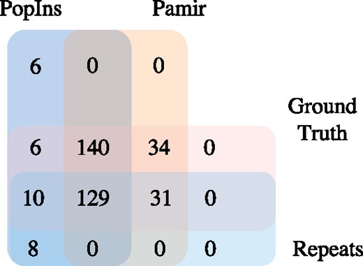
Performance comparison of PopIns and Pamir in Illumina HiSeq2500 100bp simulation dataset with 170 calls falling in repeat regions
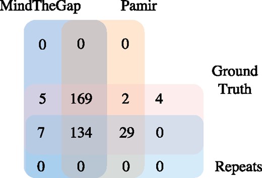
Performance comparison of PopIns and MindTheGap in Illumina HiSeq2500 100bp simulation dataset with 170 calls falling in repeat regions
3.4 Running times
Finally, we evaluated the running time of all the benchmarked software. We ran Pamir, PopIns, MindTheGap and BASIL & ANISE on a 800Mhz AMD machine with 256Gb memory with 1 thread on a high coverage simulation dataset (2*100bp error-free reads sampled from human chromosome 21 based on Illumina HiSeq2500 model at 30X coverage) until genotyping phase. Running times are given in Table 11. Pamir takes ∼3.6 times less time than BASIL & ANISE and ∼4.3 times less time than MindTheGap where PopIns takes ∼5.7 times less time than BASIL & ANISE and ∼6.8 times less time than MindTheGap. Note that PopIns is faster than Pamir, but in many cases it does not provide the full inserted sequences.
Running times of Pamir, PopIns, MindTheGap, and BASIL & ANISE on a 2*100bp simulation dataset based on HiSeq2500 model with 30X coverage
| Pamir | PopIns | MindTheGap | BASIL & ANISE |
|---|---|---|---|
| 3min 9sec | 1min 59sec | 13min 25sec | 11min 16sec |
| Pamir | PopIns | MindTheGap | BASIL & ANISE |
|---|---|---|---|
| 3min 9sec | 1min 59sec | 13min 25sec | 11min 16sec |
4 Discussion
The last few years since the introduction of HTS platforms witnessed the development of many algorithms that aim to characterize genomic structural variation. The first such algorithms focused mainly on the discovery of deletions, and other forms of complex SV, especially inversions and translocations were largely neglected due to the sequence complexity around their breakpoints and the ambiguity in mapping to these regions.
Although novel sequence insertions can be considered “simpler” than most other SV classes, their accurate characterization is still lacking due to the need for constructing either global or local de novo assembly. However, they may fail to generate long and accurate contigs due to the repeats that may occur around or within novel sequence insertions.
In this paper, we presented Pamir, a new algorithm to discover and genotype novel sequence insertions in one or multiple human genomes. Pamir uses several read signatures (one-end-anchored, read pairs, split reads, and assembly) to characterize insertions that span a wide size range. We demonstrated its performance on both simulated and real datasets and showed that it outperforms the existing tools designed for the same purpose. We believe that further development and extensive testing of the Pamir algorithm will help make the novel insertion discovery a routine analysis for whole genome sequencing studies.
Acknowledgement
We thank Alex Gawronski for proof reading and suggestions during the preparation of the manuscript.
Funding
The work was supported by an installation grant from the European Molecular Biology Organization to C.A. (EMBO-IG 2521), NSERC Discovery grant, and NSERC Discovery Frontiers grant on 'Cancer Genome Collaboratory' to F.H. P.K. acknowledges foreign collaborative research study support by The Scientific and Technological Research Council of Turkey, TÜBİTAK- BİDEB under the 2214-A programme. I.N. was supported by Vanier Canada Graduate Fellowship.
Conflict of Interest: none declared.
References
Author notes
Pınar Kavak and Yen-Yi Lin authors contributed equally to this work.

