Joint stage recognition and anatomical annotation of drosophila gene expression patterns Open Access

Abstract

1 INTRODUCTION

The mRNA in situ hybridization (ISH) provides an effective way to visualize gene expression patterns. The ISH technique can precisely document the localization of gene expression at the cellular level via visualizing the probe by colorimetric or fluorescent microscopy to allow the production of high quality images recording the spatial location and intensity of the gene expression (Fowlkes et al., 2008; Hendriks et al., 2006; L'ecuyer et al., 2007; Megason and Fraser, 2007). Such spatial and temporal characterizations of expressions paved the way for inferring regulatory networks based on spatio-temporal dynamics. The raw data produced from such experiments includes digital images of the Drosophila embryo (examples are visualized in Fig. 1) showing a particular gene expression pattern revealed by a gene-specific probe (Grumbling et al., 2006; Lyne et al., 2007; Tomancak et al., 2002, 2007). The fruit fly Drosophila melanogaster is one of the most used model organisms in developmental biology.

Fig. 1.

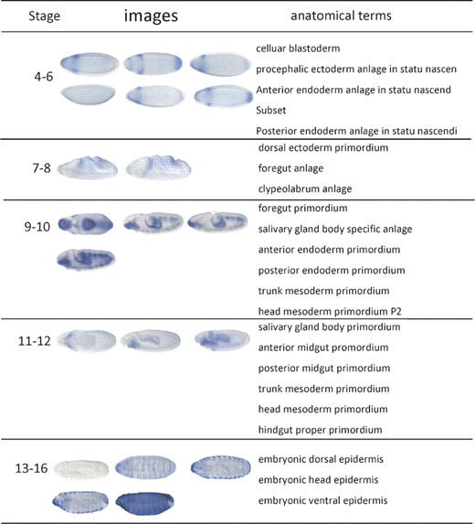
Examples of Drosophila embryo ISH images and associated anatomical annotation terms in the stages 4–6, 7–8, 9–10, 11–12 and 13–16 in the BDGP database. The darker stained region highlights the place where the gene is expressed. The darker color the region has, the higher the gene expression level is

Open in new tabDownload slide

Traditionally, such ISH images are analyzed directly by the inspection of microscope images and available from well-known databases, such as the Berkeley Drosophila Genome Project (BDGP) gene expression pattern database (Tomancak et al., 2002, 2007) and Fly-FISH (L'ecuyer et al., 2007). To facilitate spatio-temporal Drosophila gene expression pattern studies, researchers needed to solve two challenging tasks first: Drosophila gene expression pattern stage recognition (temporal descriptions) and anatomical annotation (spatial descriptions). As shown in Figure 1, Drosophila embryogenesis has been subdivided into 17 embryonic stages. These stages are defined by prominent features that are distinguishable in living Drosophila embryos (Weigmann et al., 2003). To recognize the stages of the Drosophila, embryos provide their time course patterns. On the other hand, the Drosophila gene expression patterns are often recorded by controlled vocabularies from the biologist's perspective (Tomancak et al., 2002). Such anatomical ontology terms describe the spatial biological patterns and often cross stages. What is more, because the ISH images are attached to each other collectively becoming bags of images, the corresponding stage label as well as anatomical controlled terms are the descriptions of the whole group of images instead of each individual image inside the bag. A Drosophila embryo ISH image bag belongs to only one stage, but has multiple related anatomical terms. Previously, those two tasks are tackled by domain experts. However, due to the rapid increase in the number of such images and the inevitable bias annotation by human curators, it is necessary to develop an automatic method to classify the developmental stage and annotate anatomical structure using controlled vocabulary.

Recently, a lot of research works have been proposed to solve the above two problems. They considered the stage recognition as a single-label multi-class classification problem while the anatomical annotation was treated as a multi-label multi-class classification problem. (Kumar et al., 2002) first developed an embryo enclosing algorithm to find the embryo outline and extract the binary expression patterns via adaptive thresholding. (Peng and Myers, 2004) and (Peng et al., 2007) developed new ways to represent ISH images based on Gaussian mixture models, principal component analysis and wavelet functions. Besides that, they utilized min-redundancy max-relevance to do the feature selection and automatically classify gene expression pattern developmental stages. Recently, (Puniyani et al., 2010) constructed a system (called SPEX²) and concluded that the local regression (LR) method taking advantage of the controlled term–term interactions can get the best enhanced anatomical controlled term annotation results. The LR method was proposed by Ji et al. and developed based on their previous works (Ji et al., 2008; 2010; Li et al., 2009; Shuiwang et al., 2009;). All of the above methods have provided new inspirations and insights for classifying or annotating Drosophila gene expression patterns captured by ISH. However, none of them considered doing those two tasks simultaneously. As we know, intuitively, anatomical controlled vocabulary terms provide evidence for the stage label and vice versa. For example, the early stage range is more likely annotated with the controlled terms such as ‘statu nascendi’ and ‘celluar’ than the terms ‘embryonic’ and ‘epidermis’. Therefore, besides the image–stage and image–annotation relationships which have been well studied and applied in the previous research, it is necessary to take advantage of the correlations between stage classes and annotation terms.

In this article, we propose a novel Tri-Relational Graph (TG) model that comprises the data graph, anatomical controlled terms graph, developmental stage label graph to jointly classify the stage of images and annotate anatomical terms simultaneously. Upon the TG model, we introduce a Preferential Random Walk (PRW) method to simultaneously produce image-to-stage, image-to-annotation, image-to-image, stage-to-image, stage-to-annotation, stage-to-stage, annotation-to-image, annotation-to-stage and annotation-to-annotation relevances to jointly learn the salient patterns among images that are predictive of their stage label and anatomical annotation terms. Our method achieves superior developmental stage classification performance and anatomical terms annotation results compared with the state-of-the-art methods.

We consider each image bag as a data point and extract the bag-of-word features that are widely used in computer vision research as the corresponding descriptors. Since the real object is 3D and each image can only provide 2D observation from a certain perspective, we integrate the bag-of-word features for different views. We summarize our contributions as follows:

1. This article is the first one to propose a novel solution to the questions ‘What is the developmental stage?’ and ‘What are the anatomical annotations’ simultaneously, given an unlabeled image bag.

2. Via the new TG model that we constructed, the relationships between stage label and anatomical controlled terms as well as the correlations among anatomical terms can be naturally and explicitly exploited by the graph-based semi-supervised learning methods.

3. We propose a new PRW method to seek the hidden annotation–annotation and annotation–stage relevances. Other than only using image-to-image relevance conducted by existing methods, we can directly predict the stage label and annotate anatomical controlled terms for unknown image bags.

2 DATA DESCRIPTORS

As we known, the Drosophila embryos are 3D objects. However, the corresponding image data can only demonstrate 2D information from a certain view. Since recent study has shown that incorporating images from different views can improve the classification performance consistently (Ji et al., 2008), we will use the images taken from multiple views instead of one perspective as the data descriptor. We only consider the lateral, dorsal and ventral images in our experiment due to the fact that the number of images taken from other views is much less than that of the above three views. All the images from BDGP database have been pre-processed, including alignment and resizing to 128×320 gray images. For the sake of simplicity, we extract the popular SIFT (Lowe, 2004) features from the regular patches with the radius as well as the spacing as 16 pixels (Shuiwang et al., 2009), which is shown in Figure 2. Specifically, we extract one SIFT descriptor with 128 dimensions on each patch and each image is represented by 133 (7×19) SIFT descriptors. Nevertheless, the above SIFT features cannot be directly used to measure similarity between data points (image bags), because the number of images in each image bag is different. In order to get a desired equal length descriptor to release the burden of later learning task, we need to build codebook for all extracted SIFT features first and then redo the data representations for each image bag based on the constructed codebook.

Fig. 2.

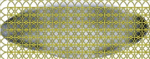
Demonstration of the regular patches. We extract one SIFT feature on one patch, where the radius and spacing of the regular patches are set to 16 pixels

Open in new tabDownload slide

2.1 Codebook construction

Usually the codebook is established by conducting the clustering algorithms on a subset of the local features, and the cluster centers are then chosen as the visual words of the codebook. In our study, we use K-means to do the clustering on the training image bags. Since the result of K-means depends on the initial centers, we repeat it with 10 random initializations from which the one resulting in the smallest objective function value is selected. The number of clusters is set to 1000, 500 and 250 for lateral, dorsal and ventral images, respectively, according to the total number of images for each view as shown in Table 1. (Other codebook sizes gave similar performance.)

2.2 Data (image bag) representations

After we get three codebooks, the images in each bag are quantized separately for each view. Features computed from patches on images with a certain view are compared with the visual words in the corresponding codebook and the visual word closest to the feature in terms of Euclidean distance is utilized to represent it. Therefore, if an image bag encompasses the images from three views, then it could be represented by three bags of words, one for each view. We concatenate the three vectors so that the images with different views (lateral, dorsal and ventral) in one bag can be represented by one vector. To be specific, Let x^l∈ℝ¹⁰⁰⁰, x^d∈ℝ⁵⁰⁰ and x^v∈ℝ²⁵⁰ denote the bag-of-words vector for images in a bag with lateral, dorsal and ventral view, respectively. The descriptor for this image bag can be represented as x=[x^l; x^d; x^v]∈ℝ¹⁷⁵⁰. Since not all the image bags enclose the images from all three views, the corresponding bag-of-words representation is a vector of zeroes if a specific view is absent. Moreover, in order to capture the variability of the number of images in each view and each bag, we normalized the bag-of-words vector to unit length. At last, each image bag is represented by a normalized vector x.

3 METHODS

In this section, we first construct a TG to model Drosophila gene expression patterns followed by proposing a novel PRW method. Using PRW on TG, we jointly make stage classification and annotate anatomical terms of Drosophila gene expression patterns.

For the Drosophila gene expression pattern data, we have n gene expression images bags X={x₁,···, x_n}, where each image bag is abstracted as a data point x_i∈ℝ^p. Each data point x_i belongs to one of K_c stage classes ={c₁,···, c_Kc} represented by y_i^c∈{0, 1}^K_c, such that y_i^c(k)=1 if x_i is classified into class c_k, and 0 otherwise. Meanwhile, each image bag x_i is also annotated with a number of anatomical ontology terms ={a₁,···, a_Ka} represented by y_i^a∈{0, 1}^K_a, such that y_i^a(k)=1 if x_i is annotated with term a_k, and 0 otherwise. Also, for convenience, we write y_i=[y_i^cT, y_i^aT]^T∈{0, 1}^K_c+K_a. Without loss of generality, we assume the first l<n image bags are already labeled, which are denoted as T={x_i, y_i}_i=1^l. Our task is to learn a function f : X→{0, 1}^K_c+K_a from T that is able to classify an unlabeled data point x_i(l+1≤i≤n) into one stage class in and to annotate it with a number of anatomical terms in at the same time. For simplicity, we write Y_c=[y₁^c,···, y_n^c], Y_a=[y₁^a,···, y_n^a], and Y=[y_1,···, y_n]. As introduced in Section 1, the stage class and anatomical terms have some relations. We utilize the following affinity matrix to model their interrelations, R∈ℝ^K_c×K_a, where R(i, j) indicates how closely class c_i and term a_j are related. In this work, we compute it as

(1)

where is the i-th row of Y_c and is the j-th row of Y_a. Throughout this article, we denote a vector as a bold lowercase character and a matrix as an uppercase character. We denote the i-th entry of a vector v as v(i), and the entry at the i-th row and j-th column of a matrix M as M(i, j). ||v|| denotes the Euclidian norm of vector v. And the inner product of two vector v₁ and v₂ is defined as <v₁, v₂>=v₁^Tv₂.

3.1 The construction of TG

Given the dataset X, pairwise similarity W_X∈ℝ^n×n between data points can be computed using the Gaussian kernel function,

(2)

where the vector x is calculated using bag-of-word features for one image bag. Regarding the parameter σ, we resort to self-tuning method (Zelnik-Manor and Perona, 2004). W_X(i, j) indicates how closely x_i and x_j are related. From W_X, a graph _X=(_X, _X) can be induced, where _X=X and _X⊆_X×_X. And we use kNN graph. To be specific, we connect x_i, x_j if one of them is among the other's k nearest neighbor and define the value of the edge connecting them by Equation (2). Because _X characterizes the relationships between data points, it is usually called as data graph, such as the middle subgraph in Figure 3. Existing graph-based semi-supervised learning methods (Kang et al., 2006; Zha et al., 2008) only make use of the data graph, on which the class label information is propagated.

Fig. 3.

The TG constructed from the gene expression data. Solid lines indicate affinity between vertices within in a same subgraph, dashed lines indicates associations between vertices in two different subgraphs

Open in new tabDownload slide

Different from conventional single-label classification learning problem in which classes are mutual exclusive, the anatomical terms are interrelated with one another. Again, we resort to cosine similarity to calculate the controlled term affinity matrix W_A, where W_A(i, j) indicates the correlation between a_i and a_j. Thus, a graph _A=(_A, _A) is induced, where _A= and _A⊆_A×_A. We call _A as annotation label subgraph, which is shown as the right subgraph in Figure 3. Similarly, stage classification label graph shown as the left subgraph in Figure 3, _C=(_C, _C) can be constructed from stage classification labels, where _C= and _C⊆_C×_C, where we define the value of the edge connecting two stage labels as W_C(i, j)=‖S_bi−S_bj‖_F, where ‖ ‖_F means Frobenius norm and S_bi denotes the between class scatter matrix for stage i. Connecting _X and _A by the annotation associations via the green dashed lines, connecting _X and _C by the class associations via the blue dashed lines and connecting _C and _A by the stage-term association via the purple dashed lines, we construct a TG as following:

(3)

which is illustrated in Figure 3. Obviously, the subgraph _AX=(_X, V_A, _XA) connects G_X and G_A, whose adjacency matrix is Y_a^T. Similarly, the adjacency matrix of _CX=(_X, _C, _XC) is Y_c^T. The subgraph (_C, _A, _CA) characterizes the associations between stage classes and anatomical terms whose adjacency matrix is R defined in Equation (1).

In contrast to existing graph-based semi-supervised learning methods that only use information conveyed by _X, we aim to simultaneously classify and annotate an unlabeled data point using all the information encoded in . Since all data points (gene expression image bags), stage terms and annotation terms are equally regarded as vertices on , our task is to measure the relevance between a class/anntotation term vertex and a data point vertex. As each class/annotation term has a set of associated training data points, which convey the same biological record information as the class/annotation term, we consider both a class/annotation term vertex and its labeled training image bag vertices as a group set,

(4)

which is illustrated as the vertices with orange boundary in 3. As a result, instead of measuring vertex-to-vertex relevance between a class/annotatation term vertex and an unlabeled data point vertex, we may measure the set-to-vertex relevance between the group set and the data point. Motivated by Brin and Page (1998); Tong et al. (2006), we consider to further develop standard random walk and use its equilibrium probability to measure the relevance between a group set and an unlabeled data point.

3.2 Preferential random walk

Standard random walk on a graph W can be described as a Markov process with transition probability M=D⁻¹W, where d_i=∑_jW(i, j) is the degree of vertex i and D=diag(d₁,···, d_n). Clearly, M^T ≠ M and ∑_jM(i, j)=1. When W is symmetric, it corresponds to an undirected graph. When W is asymmetric, it corresponds to a directed graph and d_i is the out degree of vertex i. Let p^(t) be the distribution of the random walker at time t, the distribution at t+1 is given by p^(t+1)(j)=∑_ip^(t)(i)M(i, j). Thus, the equilibrium (stationary) distribution of the random walk p^*=p^(t=∞) is determined by M^Tp^*=p^*. It is well known that the solution is simply given by p^*=We/(∑_id_i)=d/(∑_id_i), where d=[d₁,···, d_n]^T.

It can be seen that the equilibrium distribution of a standard random walk is solely determined by the graph itself, but independent of the location where the random walk is initiated. In order to incorporate label information, we propose the following PRW:

(5)

where 0≤α≤1 is a fixed parameter, and h, called preferential distribution, is a probability distribution such that h(i)≥0 and ∑_ih(i)=1 . Equation (5) describes a random walk process in which the random walker hops on the graph W according to the transition matrix M with probability 1 − α, and meanwhile it takes a preference to go to other vertices specified by h with probability α. The equilibrium distribution of PRW in Equation (5) is determined by p^*=(1 − α )M^Tp^*+αh, which leads to:

(6)

Due to Perron-Frobenius theorem, the maximum eigenvalue of M is less than max_i ∑_jM(i, j)=1. Thus, I−(1 − α)M^T is positive definite and invertible. Equation (5) takes a similar form to two existing works: random walk with restart (RWR) method (Tong et al., 2006) and PageRank algorithm (Brin and Page, 1998). In the former, h is a vector with all entries to be 0 except one entry to be 1 indicating the vertex where the random walk could be restarted; while in the latter, h is a constant vector called as damping factor (Brin and Page, 1998). In contrast, the preferential distribution vector h in Equation (5) is a generic probability distribution, which is flexible thereby more powerful. Most importantly, through h we can assess group-to-vertex relevance, while RWR and PageRank methods measure vertex-to-vertex relevance.

Similar to RWR (Tong et al., 2006), when we set the h to be a probability distribution in which all the entries are 0 except for those corresponding to _k, p^*(i) measures how relevant the k-th group is to the i-th vertex on .

3.3 Preferential random walk on TG

In order to classify and annotate unlabeled data points using the equilibrium probabilities in Equation (6) of the PRW on TG, we need to construct the transition matrix M and the preferential distribution h from .

Construction of the transition matrix M:

Let

(7)

where M_X, M_C and M_A are the intrasubgraph transition matrices of _X, _C and _A respectively, and the rest six sub-matrices are the intersubgraph transition matrices among _X, _C and _A. Let β₁∈[0, 1] be the jumping probability, i.e. the probability that a random walker hops from _X to _C and vice versa. And let β₂∈[0, 1] be the jumping probability from _X to _A or vice versa. Therefore, β₁ and β₂ regulates the reinforcement between _X and one of the other two subgraphs. When both β₁=0 and β₂=0, the random walk are performed independently on _X, which is equivalent to existing graph-based semi-supervised learning methods only using the data graph _X. Similarly, we define λ as the jumping probability from _C to _A or vice versa.

During a random walk process, if the random walker is on a vertex of the data subgraph which has at least one connection to the label subgraph, such as vertex x₁ in Figure 3, she can hops to the class label or annotation subgraph with probability β₁ or annotation subgraph with probability β₂, or stay on the data subgraph with probability 1 − β₁ − β₂ and hop to other vertices of the data subgraph. If the random walker is on a vertex of the data subgraph without a connection to the class label or annotation subgraph, she stays on the data subgraph and hops to other vertices on it as in standard random walk process. To be more precise, let d_i^Y_cT=∑_jY_c^T(i, j), the transition probability from x_i to c_j is defined as following:

(8)

Similarly, let d_i^Y_c=∑_jY_c(i, j), the transition probability from c_i to x_j is:

(9)

Following the same definition, the rest four inter-subgraph transition probability matrices are defined as:

(10)

(11)

where d_i^Y_aT=∑_jY_a^T(i, j) and d_i^Y_a=∑_jY_a(i, j), and

(12)

(13)

where d_i^RT=∑_jR^T(i, j) and d_i^R=∑_jR(i, j).

Let d_i^X=∑_jW_X(i, j), d_i^Y=∑_jY(i, j), d_i^Q_a=∑_jQ_a(i, j), d_i^Q_c=∑_jQ_c(i, j) where Q_a=R+Y_a and Q_c=R^T+Y_c.

The data subgraph intra transition probability from x_i to x_j is computed as:

(14)

Similarly, let d_i^A=∑_jW_A(i, j), the annotation label subgraph intra transition probability from a_i to a_j is:

(15)

let d_i^C=∑_jW_C(i, j), the classification label subgraph intra transition probability from c_i to c_j is:

(16)

It can be easily verified that, ∑_jM(i, j)=1, i.e. M is a stochastic matrix.

Construction of the preferential distribution H:

the preferential distribution vector specifies a group of vertices to which the random walker prefers to moving in every iteration step. The relevance between this group and an vertex is measured by the equilibrium distribution of the random walk process. Therefore, we construct K=K_c+K_a preferential distribution vectors, one for each semantic group G_k:

(17)

where h^(k)(i)=1/∑_iy_i(k) if y_i(k)=1 and h^(k)(i)=0, otherwise; h^(k)(i)=1, if i=k, γ∈[0, 1] controls how much the random walker prefers to go to the data subgraph and other two subgraphs , . It can be verified that ∑_ih^(k)(i)=1, i.e, h^(k) is a probability distribution. Let I_K be the identity matrix of size K×K, we write

(18)

PRW on TG:

given the TG of a dataset, using the transition matrix M defined in Equation (7) and the preferential probability matrix H defined in Equation (18), we can perform PRW on the TG. According to Equation (6), its equilibrium distribution matrix P^* is computed as:

(19)

P^*=[p₁^*,···, p_K^*]∈ℝ^(n+K)×K, and p_k^* is the equilibrium distribution of the PRW taking the k-th semantic group as preference. Therefore, p_k^*(i) (l+1≤i≤n) measures the relevance between the k-th class and an unlabeled image bag x_i. We can predict the stage class from the sub-matrix P_nc^* by Equation (20) and annotate the controlled terms for x_i using the adaptive decision boundary method (Wang et al., 2009) on the submatrix P_na^* by Equation (21).

(20)

(21)

Since the stage prediction is a single-label classification problem, we select the stage label y(i)^c* with the maximum probability as the stage label for image bag x_i.

(22)

where is the i-th row vector of matrix P_nc^*. Therefore, we can do the stage classification and anatomical controlled term annotation simultaneously.

4 DATA REFINEMENT

In this section, we will introduce the details of the data used in our experiment. Drosophila embryogenesis has 17 stages, which are divided into 6 major ranges, i.e. stages 1–3, 4–6, 7–8, 9–10, 11–12 and 13–16 (the stage 17 is usually studied individually), in the BDGP database (Tomancak et al., 2002). Each image bag is labeled with one stage term and many controlled vocabulary terms. The total number of anatomical controlled vocabulary terms is 303.

We used the following way to refine the dataset. First, we only keep the image bag data with lateral, dorsal and ventral view information. And then, we eliminate six common annotation terms, that is, ‘no staining, ubiquitous, strong ubiquitous, faint ubiquitous, maternal, rapidly degraded’, which can be regarded as outliers because they can neither provide stage-specific information nor record anatomical structures. After that, we remove the anatomical terms whose data sample is <50. We ignore the stage 1–3 data since the number of anatomical terms after the above procedure becomes 2, too small to be compared with other stages. And finally we get 79 anatomical annotation terms in total that we will consider to annotate the unlabeled image bag.

We refine the data mainly based on the following two reasons. On one hand, the annotation terms which appear in too few image bags are statistically too weak to be learned effectively. On the other hand, since we will use 5-fold cross-validations in our experiments, we have to guarantee there is at least one data point associated with each anatomical term in each fold. Moreover, in order to balance the number of image bags for different stages, we randomly sample 500 image bags as the data points for each stage. At last, the summary of the refined dataset is shown in Table 1.

5 EXPERIMENT

In this section, we will conduct experiments to evaluate PRW empirically on the refined dataset and compare it with other state-of-art classification methods. Since our method can do joint classification, in order to evaluate the benefit of joint learning, we compare its performance with that of the state-of-art multiclass single label or multiclass multilabel algorithms which can only handle either stage classification or anatomical term annotation problem. Our procedure is to train our model with stage labeled and anatomical term annotated image bags. All testing image bags are unlabeled with developmental stage and unannotated with anatomical controlled terms.

5.1 Experimental setup

When constructing PRW on TG, we used kNN graph setting k=9. We used ‘inverse’ 5-fold cross-validation to determine the values of the following five parameters, that is, using 1-fold for training and using the remaining 4-folds for testing to mimic the scenario in the real application where the number of training data is much less than the testing data. In our experiment, we found that the following five parameters are not sensitive in certain ranges with good performances. β₁, β₂ and λ controls the jumping between different subgraphs and cannot affect the result much if they are assigned in the range of (0.1, 0.45). α controls initial preference of the random walker and will get stable result if it is assigned in the range of (0, 0.1). γ controls how much the random walker prefers to go to the data subgraph or to go to two other subgraphs and it is usually in the range of (0.1, 0.3).

Besides those parameters, we also need to initialize the stage as well as anatomical controlled terms for the testing image bag x_i, where i=l+1,…, n, l is the number of training image bag. In our experiment, we used k-nearest neighbor (KNN) method to do the initializations for both stage classification and anatomical term annotations tasks because of its simplicity and clear intuition. To be specific, we use k=1 and we abbreviate it as 1NN. Our joint classification framework will self-consistently amend the incorrect labels for stage and controlled terms. We perform 10 random splits of the data and report the average performance over the 10 trials. Please note that, in each trial, we still do ‘inverse’ 5-fold cross validation and record the average performance result as the result of that trial.

5.2 Image bag stage classification

Drosophila gene expression pattern stage categorization is a single-label multi-class problem. We compare the result of our method with that of support vector machine (SVM) with radial basis function (RBF) kernel (Chang and Lin, 2001). We use the optimal parameter values for C and γ got from cross-validation as well. We also compare the classification result of 1NN that we use to do the initialization. We assess the classification in terms of the average classification accuracy and the average confusion matrices. Since the data that we used is class balanced, the mean value of the entries on the diagonal of the confusion matrix is also the average classification accuracy. From the resulting average confusion matrices shown in Figure 5, we can see that the average prediction accuracy of our method is better than that of the other two state-of-art methods, especially in the last stage 13–16, where the number of anatomical terms is greatly larger than that of the other stages.

5.3 Image bag controlled vocabulary terms annotation

Besides the stage classification task, we also validate our method by predicting the anatomical controlled terms for the Drosophila gene expression patterns, which can be considered as a multi-class multi-label classification problem. The conventional classification performance metrics in statistical learning, precision and F1 score, are utilized to evaluate the proposed methods. For every anatomical term, the precision and F1 score are computed following the standard definition for the binary classification problem. To address the multi-label scenario, following Tsoumakas and Vlahavas (2007), macro and micro average of precision and F1 score are used to assess the overall performance across multiple labels. We compared four state of art multi-label classification methods: local shared subspace (LS) (Ji et al., 2008), local regression (LR) (Ji et al., 2009), harmonic function (HF) (Zhu et al., 2003) and random walk (RW) (Zhou and Schölkopf, 2004). All of them are proposed recently to solve the multilabel annotation problem. In addition, we compare the results of 1NN as well. For the first three methods we use the published codes posted on the corresponding author's websites. And we implement the RW method following the original work (Zhou and Schölkopf, 2004). For HF and RW methods, we follow the original work to solve the multilabel annotation only. Therefore, we only evaluate those two methods on data subgraph and annotation label subgraph without using any information derived from the classification label subgraph such as the stage–term correlation. Table 2 shows the average anatomical annotation performance of 79-term dataset. Compared to the above five stat-of-the-art methods, our method has the best results by all metrics. Figure 6 illustrates the average Micro F1 score of our method, 1NN, LS, LR, RW and HF approaches for all the anatomical terms on 79-term dataset. And again, our method consistently achieves best performance for most of the anatomical controlled terms.

5.4 The advantage of joint learning

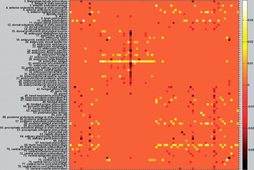
Unlike the traditional work, our proposed method can take advantage of all the information to do the stage classification and anatomical term annotation simultaneously. Therefore, when the number of training data is scare, we can resort to both intrarelations and interrelations to make the decision for stage classification and anatomical controlled term annotation simultaneously. When there are strong correlation between those two tasks, we expect that the performance of both tasks will be enhanced by joint learning work than treating them individually and independently. Figure 4 shows the pairwise label correlations of the 79 terms and stage–term correlations between 5 stages and 79 terms. As highlighted by purple arrows, we can observe that there are high pairwise correlations between the terms ‘embryonic brain’,‘ventral nerve cord’ as well as ‘embryonic/larval muscle system’. Moreover, all the above three terms have high correlations with the stage 13–16, which can provide strong evidence that the given testing image bag could belong to the last developmental stage besides the induction from the data graph only. If our joint classification framework annotates it with all those three terms, although from the data similarity we cannot get strong evidence for the stage prediction, we can take advantage of the term–term as well as term–stage high correlations to adjust its stage to stage 13–16. In other words, relevant anatomical terms could help us to predict the stage label since they provide the spatial and temporal information of local structure corresponding to a specific embryo development stage. Nevertheless, not all anatomical terms will definitely benefit stage classification, which is consistent with our stage classification result. From Figure 5, we can see that our method may have competitive result compared with SVM with respect to some certain stage. However, given more anatomical term information, the performance of our method will gradually outperform the other methods, especially for the prediction result of stage 13–16.

Fig. 4.

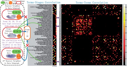
The middle part demonstrates the terms–stages correlation and the right part shows the terms–terms correlation of 79 terms. The stage unknown test data shown in the left part is classified correctly as Stage 13–16, because of the strong correlation between the predicted stage and its predicted anatomical terms and vice versa, NOT the similarity of its first and second nearest neighboring data induced from the data graph only

Open in new tabDownload slide

Fig. 5.

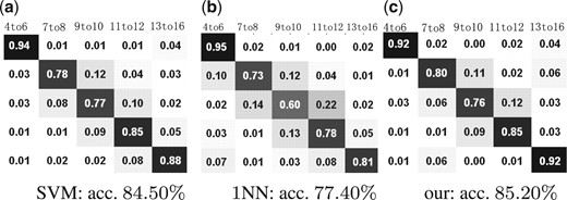
Stage classification results in terms of confusion matrices on 79-term dataset: (a) the confusion matrix calculated by SVM (b) the confusion matrix calculated by 1NN. (c) the confusion matrix calculated by our method. (a) SVM: acc. 84.50%; (b) 1NN: acc. 77.40%; (c) our: acc. 85.20%

Open in new tabDownload slide

Fig. 6.

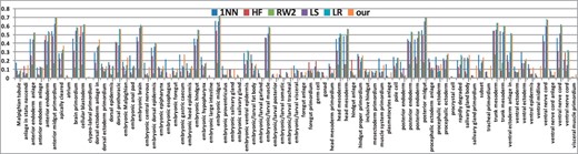
The Avg. Micro F1 score of five methods on each term in 79-term dataset. (It is better to be viewed in colorful and zoomed in mode.)

Open in new tabDownload slide

5.5 The more meaningful asymmetric correlation matrix

When we build the TG, at first, we assume the term–term correlation and stage–term correlation are both symmetric, since we used cosine similarity to represent their correlations. However, the above assumption does not always hold in the real data. In Drosophila embryo gene expression images, we found that the conditional probability of the occurrence of term ‘ventral nerve cord’ given term ‘embryonic brain’ is higher than that of the ‘embryonic brain’ given ‘ventral nerve cord’, which satisfies the biology meaning that ventral nerve cord occurs earlier than embryonic brain. After learning, our method can automatically discover the above hidden asymmetric correlation information, that is,

(23)

In order to see the learned asymmetric term–term correlation more clearly, in Figure 7, we show the difference matrix got by P_aa^*−P_aa^*T. Taking those more accurate asymmetric correlation into consideration, our method can potentially improve both stage classification and anatomical annotation results even more.

Fig. 7.

The learned difference matrix. (It is better to be viewed in colorful and zoomed in mode.) In order to see the asymmetric entries more clearly, we plot P_aa^*−P_aa^*T. After PRW, the entries marked as brighter square have higher conditional probability (positive correlation) than its counterpart which is marked as darker color. This asymmetric reflects more accurate term–term correlation than the original symmetric assumption

Open in new tabDownload slide

6 CONCLUSION

In this article, we proposed a novel TG model to learn the task interrelations between stage recognition and anatomical terms annotation of Drosophila gene expression patterns. The standard bag-of-word features and three major views (lateral, dorsal and ventral) were used to describe the 3D Drosophila images. A new PRW method was introduced to simultaneously propagate the stage labels and anatomical controlled terms via TG model. Both stage classification and anatomical controlled term annotation tasks are jointly completed. We evaluated the proposed method using one refined BDGP dataset. The experimental results demonstrated in the real application, when the number of training data is scarce, our joint learning method can achieve superior prediction results on both tasks than the state-of-the-art methods. What is more, we can discovery more accurate asymmetric term–term correlation, which can potentially improve the results of both tasks even more.

ACKNOWLEDGEMENT

The author would like to thank Dr Sudhir Kumar for his help in data collection.

Funding: [This research was supported by National Science Foundation Grants CCF-0830780, CCF-0917274, DMS-0915228 and IIS-1117965].

REFERENCES