


Abstract
Motivation: The recent development of high-throughput drug profiling (high content screening or HCS) provides a large amount of quantitative multidimensional data. Despite its potentials, it poses several challenges for academia and industry analysts alike. This is especially true for ranking the effectiveness of several drugs from many thousands of images directly. This paper introduces, for the first time, a new framework for automatically ordering the performance of drugs, called fractional adjusted bi-partitional score (FABS). This general strategy takes advantage of graph-based formulations and solutions and avoids many shortfalls of traditionally used methods in practice. We experimented with FABS framework by implementing it with a specific algorithm, a variant of normalized cut—normalized cut prime (FABS-NC′), producing a ranking of drugs. This algorithm is known to run in polynomial time and therefore can scale well in high-throughput applications.
Results: We compare the performance of FABS-NC′ to other methods that could be used for drugs ranking. We devise two variants of the FABS algorithm: FABS-SVM that utilizes support vector machine (SVM) as black box, and FABS-Spectral that utilizes the eigenvector technique (spectral) as black box. We compare the performance of FABS-NC′ also to three other methods that have been previously considered: center ranking (Center), PCA ranking (PCA), and graph transition energy method (GTEM). The conclusion is encouraging: FABS-NC′ consistently outperforms all these five alternatives. FABS-SVM has the second best performance among these six methods, but is far behind FABS-NC′: In some cases FABS-NC′ produces over half correctly predicted ranking experiment trials than FABS-SVM.
Availability: The system and data for the evaluation reported here will be made available upon request to the authors after this manuscript is accepted for publication.
Contact: [email protected]
1 INTRODUCTION
Automated microscopy is increasingly used in drug discovery, especially predicting the toxicity of new drugs (Perlman and Altschuler, 2004). The so-called high-content screening (HCS) has greatly enhanced investigators' capability of discerning the response of cells treated by various drugs (Conrad and Gerlich, 2010; Denner et al., 2008; Feng et al., 2009; Lang et al., 2006; Mitchison, 2005a; Nichols, 2007; Taylor and Hsaskins, 2007). HCS accomplishes this by analyzing phenotypic features of the cells from tens of thousands cell images produced by HCS. In addition, the decreasing cost of such a method means a wide-spread application (Lin et al., 2010). HCS employs cell imaging assays, tagged with fluorescent dyes—each field of cells contains these tags for its different macromolecules. Automated microscopy is performed to produce a large amount of visual information.
There are three steps during this process (Mitchison, 2005a; Yarrow et al., 2003): fluorescence-tagging, automated microscopy and identification and measurement of target phenotypic feature(s) for further analysis. The analysis step usually poses the most challenge. To extract meaning out of a gigantic image database, traditional tools usually need to be tailored to specific known phenotype's features, instead of unknown yet more informative differences. For example, it has been reported that applying an analysis method that only distinguishes phenotypic changes in cellular level misses on the detecting meaningful morphological modification on subcellular structures (Taguchi et al., 2007; Zhou and Wong, 2006).
In high-throughput drug screening assays, typically a quantity, such as normalized intensity of a reporter fluorescent protein (Morelock et al., 2005), is assumed to be measurable. Differences between samples of two distinct cell populations (such as treated versus untreated) are estimated and tested for significance. Methods using statistics like Z′-factor (Zhang et al., 1999) to evaluate reliability of the measurements have been developed. Comparison of the difference is usually done by performing a multivariate F-test to test whether two populations are distributed differently. But F-test may introduce high errors when the distributions are not normal, which is expected to be the case in many types of cell responses. Moreover, in image-based assays, the use of a measurable quantity is no longer applicable when this quantity is not straightforward to obtain directly and the measurement itself can never be perfect. For example, to measure the composition of morphological subtypes of mitochondria requires pattern recognition algorithms to accurately detect and quantify target events (Peng et al., 2011). Though many advanced algorithms have been developed for years, these pattern recognition algorithms usually require non-trivial tuning and optimization for each study because they may generalize poorly, sometimes not even generalize within a well, due to noise and systematic bias introduced during the sample preparation and imaging process steps, inducing additional overhead when attempts are made to scale up the assay to high throughput.
Another challenge is when a multiplex approach is required, where multiple independent quantities are measured for each single cell. In these cases, response of each single cell will be a multi-dimensional vector. How to measure difference between these vectors become an issue because simple Euclidean distance in the multi-dimensional space may not serve the need. One solution is to come up with an appropriate ‘metric’ to convert multi-dimensional vectors into a scalar that reflects the difference. There is, however, no generally applicable solution about how to come up with this metric. Usually, one or more dimensions in the vector come from an imperfectly measured quantity, such as one that requires advanced pattern recognition in order to automatically extract, as discussed in the previous paragraph. Another issue is that our observation is the result of sampling, which inevitably introduces sampling errors and is further complicated by possible heterogeneous responses by cells (Altschuler and Wu, 2010).
The focus of this research is to address the issues mentioned above for the application of HCS in drug ranking. Drug ranking refers to the ordering of a group of different drugs according to their effectiveness by certain criteria. One of the most used criteria is the relative toxicity among drugs (Paull et al., 1992). Ideally, this provides the important scale to assess relative merit of each candidate drug. However, each cell responds to a certain drug differently, thus making the outcome of any ranking highly dependent on sampling and noise. A conspicuous example is the fragmentation of cells or organelles: the intact and the completely fragmented states are easy to recognize while the degree of partial fragmentation is difficult to gage, thus often involving human experts and time-consuming manual processes. This is infeasible for high-throughput screening such as HCS (Lin et al., 2010; Peng et al., 2011).
Our objective is to develop an efficient and accurate ranking measure (metric learning) that can be used to order candidate drugs according to their effectiveness. To this end, we developed a framework called Fractional Adjusted Bi-partitional Score (FABS). This general strategy, introduced here for the first time, takes advantages of graph-based formulations and solutions and avoids many shortfalls of traditionally used methods in practice. We use such a scheme because graph-based construction works well in several areas of data mining (Washio and Motoda, 2003), machine learning (Jordan, 1996) and image processing (Hochbaum, 2001), whereas a recent publication (Lin et al., 2010) also confirms its usefulness in the HCS context.
In order to apply our FABS to the images, we use a feature extraction tool first presented in (Peng et al., 2011). This tool takes cell images and output several vectors that represents important geometric and other features of the target images—these vectors are then used as inputs for getting FABS.
One feature of FABS is that it has, as part of the input and as training data, extreme cases labeled as positive and negative controls, which in our case are the intact and the completely fragmented states mentioned previously. The algorithm does not involve any training from in-between cases, which are hard to come by. This completely sidesteps the common problem of a laborious and time-consuming annotation step, performed by experts to assess the relative merit of drugs for a small sample of images used as a training group. Furthermore, our measure takes the advantage of high-volume nature of the dataset, using all available images for computation of FABS for each drug. This reduces the effect of noise and sampling bias. This framework can potentially be used for any task that requires to quantify subtle and implicit differences between populations of high-dimensional feature vectors. By formulating the problem as a biparition problem as in FABS, there is no need to solve an image-based drug ranking problem as a regression problem. Our preliminary formal analysis of FABS shows that the expected error and variance of the estimated scores by FABS will be within a manageable range given the classification error by the bipartition.
To empirically evaluate our framework, we use a model of (NC′) and the respective algorithm recently introduced by Hochbaum (2010c). That algorithm runs efficiently and is furthermore combinatorial. This latter feature differentiates it from ref. (Lin et al., 2010) in which a spectral techniques is used to achieve a bipartitioning. Combinatorial solutions are superior than spectral ones in several regards such as being more efficient and accurate (Hochbaum, 2010b,c), as shown in our experimental results.
2 METHODOLOGY
This section presents a general framework for quantifying the difference in morphological composition between populations of cells. The proposed framework utilizes a procedure named FABS- , where stands for a bipartition algorithm and FABS stands for (FABS). We show that using certain graph, theoretical formulations for the bipartition algorithm avoids many shortfalls of the methods used in practice. Its importance lies in teasing apart cell groups based on morphological composition and in detecting whether or not such differences exist.
As previously mentioned, we use a feature extraction tool, capable of processing cell images with different dimensionalities (from static 2D to animated 3D with multiple channels) to generate high-dimensional (in our experiments, 134 D) output vectors, called feature vectors. Each feature vector, corresponds to an image of a single cell and contains measurements for the image characteristics, such as the intensity of the image, the shape of a particular object in the image, etc. Each group of cell images (and their corresponding feature vectors) can be associated with a certain population (e.g. populations representing cells to whom a certain drug has been applied).
The method proposed in this section, FABS-, is capable of receiving—as input—the feature vectors from cells representing different populations and detecting and quantifying the differences between these populations. For example, given the features extracted from the mitochondrial images of two populations of cells, one derived from diseased tissues and the other from healthy tissues, FABS- will tell us to what extent the fragmentation levels of their mitochondria are different and estimate the significance of the difference.
We then perform FABS- on the processed feature vectors. The input to FABS- is the processed feature vectors by principal component analysis (PCA) to reduce dimensionalities of the original data, each of which belongs to a certain population set, namely, Pi, and training data. The training data consists of feature vectors belonging to two populations on the opposite ends of the spectrum, R1 and R2. These two population sets represent positive and negative controls, which in this experiment are the completely fragmented and the completely intact mitochondria cell populations.
Computation of FABS-, the details of which will be discussed shortly, consists of three steps: The first step is to construct a graph from the input data. The second step is to apply a blackbox algorithm () to find a bipartition on the resulting graph. The third step is to recover a scalar score for each population, based on the fraction of the cases that fall in the side of the partition boundary (cut) that contains positive controls. The blackbox can be any appropriate bipartitioning algorithm available. The algorithm we propose to use for the blackbox solves the normalized cut prime (NC′) problem (Hochbaum, 2010b). We refer to this algorithm as NC′. We shall see in the ‘Results’ section that this bipartitioning algorithm, in the context of FABS- (FABS-NC′), outperforms Support Vector Machine (SVM) algorithm (FABS-SVM). This overall framework provides a flexible general strategy for quantifying the differences among population groups.
The major advantages of FABS- include:
In what follows we describe the three steps of FABS- in more details.
it is capable of efficiently processing the high-dimensional input data acquired from the images using feature extraction tool from Peng et al. (2011);
the generated output is one-dimensional, in that a single scalar score is generated for each population of multidimensional vectors. As such, the difference between the scores can be used to quantify population differences in an unambiguous way;
the calculation of the output scores is done in a way that reduces the effects of outliers in distinguishing cell populations;
unlike many statistical tests, it does not assume any underlying distribution for the populations;
the labeled training data set required is minimal and easily obtainable, requiring minimum intervention from the experts; and
it scales well in high-throughput applications.
2.1 The FABS-![graphic]() Algorithm
Algorithm
Step 1: graph construction
As mentioned previously, the input to FABS- consists of n (pre-processed) feature vectors, V={v1,…, vn}, each associated with an HCS image, obtained after feature extraction and PCA pre-processing. This input includes k population sets, {P1,…, Pk}. Each population set in this case represents a set of feature vectors corresponding to cells treated with a certain drug. Each feature vector vi belongs to one of the population sets, indicating in this case what drug has been applied to the particular cell the vector is representing. The input also contains two training sets {R1, R2}, representing the extreme cases such as the completely fragmented and the completely intact mitochondria cell populations. In the graph construction step of FABS-, an undirected graph G=(V, E, l, w) is created, where each node vi∈V corresponds to a feature vector. The set of all possible pairs correspond to the set of edges of the graph E=V×V that form a complete graph. Each feature vector vi is labeled with lvi, which is the index of the population set it belongs to. The labeling function, lvi, assigns a mapping from each feature vector, vi, to its corresponding population set, determining which population it belongs to. A weight function w: V×V →ℜ+ associates with each pair of nodes {i, j} (an edge) its encoding connection strength, or the similarity strength between the two nodes. For each edge [i, j], the weight wij and the distance between the two points vi and vj have the relationship: one goes up as the other goes down (or vice versa)—this also means that wij and the similarity between vi and vj both go up or down together. Several distance measures can be used for this purpose, among them, Euclidean, city block and Minkowski distances. Notice that constructing these similarity measures makes the dimensionality of the vectors irrelevant to our algorithm.
Step 2: bipartitioning the graph using NC′
 , where
  . The capacity of a cut
 , is defined as:
As previously mentioned, in the second step of FABS-, we use a blackbox algorithm to find a bipartition on the graph. A bipartition algorithm aims at finding the cut that separates the graph into S and  , according to some underlying objectives. There are many different objectives that can be selected. For instance, the bipartition algorithm for the well-known minimum cut problem is defined with the goal of separating the graph into S and
  such that
  is the minimum among all possible non-empty subsets S and
  . Since the goal is to obtain a bipartition for the FABS- calculation process, any bipartition algorithm can be used as a blackbox. However, an extra requirement has to be imposed (either by the internal working of the algorithm or by an external constraint) listed as follows.
Requirement 1.
All positive controls R1 must be in S (or  ) and all negative controls R2 must be in
  (or S).
For a particular blackbox implementation of FABS- in Step 2 of Algorithm 1, we choose the previously mentioned bipartitioning algorithm, called NC′, and adjust it to guarantee that the constraint listed in Requirement 1 is satisfied. The resulting FABS-NC′ is semi-supervised in nature and incorporates all information of the corresponding graph. The NC′ problem is defined as finding  on a given graph. This objective combines the goal of minimizing the similarity between the two parts of the bipartition, the quantity
  , with the goal of maximizing the similarity between the elements of S. For a graph G=(V, E), we denote NC
 . An efficient algorithm for this problem was given in (Hochbaum, 2010a,b,c).
The polynomial time algorithm described in (Hochbaum, 2010b) for NC′ was based on showing that solving NC′ is equivalent to solving a certain parametric s,t-cut problem. In an s,t-cut problem a node of a graph s is required to be on one side of the bipartition, whereas the node t is required to be on the opposite side.
In the adaptation of the parametric s,t-cut algorithm for the FABS- framework, the positive and negative control data are used as seed nodes that are forced to join s and t in the graph. This is achieved through setting the nodes in R1 to be ‘infinitely similar’ to the source node s, and the nodes of R2 to be ‘infinitely similar’ to the sink node t. In terms of the graph that means that we add edges of infinite weight between the source node s and all nodes in R1, and edges of infinite weight between the nodes of R2 and t.
Since NC′ can be solved in the running time of a minimum s,t-cut problem (Hochbaum, 2010b), our FABS-NC′ implementation is efficient, solving in polynomial time. We later compare the performance of FABS-NC′, with FABS-SVM, where the bipartitioning algorithm used is SVM, whose objective is to find a high-dimensional hyperplane that is as wide as possible to separate data of different labels (Cristianini and Shawe-Taylor, 2000).
Step 3: computing FABS scores
 . In the third step of FABS-, a scalar score, FABSPi, is calculated for each population set Pi. FABSPi is the fraction of the number of feature vectors in Pi that fall in the set S, to the total number of feature vectors in Pi. Formally,
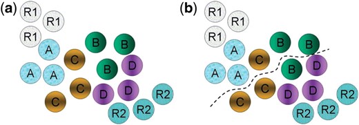
(a) The input with the feature vectors of images associated with positive and negative controls R1 and R2 and four different drugs drug A, drug B, drug C and drug D; (b) The bipartition boundary after the cut is found: if R2 contains negative controls, such as the completely fragmented state of mitochondria for toxicity criterion, while R1 contains positive controls, representing cells in a desired normal healthy state with mitochondria rescued from the completely fragmented, then FABSdrug A=1, FABSdrug B=2/3, FABSdrug C=1/3, and FABSdrug D=0. Our ranking of the drugs will be: drug A >> drug B >> drug C >> drug D, where x >> y indicates that x is more effective than y
The entire procedure is summarized in Algorithm 1.

2.2 Significance test
One can further use the FABS scores to test statistical significance of the difference between the effects of two drugs. The idea is to apply bootstrapping to obtain FABS scores from a large number of resampling trials and then perform hypothesis test on the difference of the distributions of FABS. Algorithm 2 gives the test procedure, which takes resulting FABS from repeated experiment and calculate P-values from a t-test for each drug. The obtained P-value is then transformed into a log score −logp.
To see if t-test is appropriate, there are several important assumptions to check. First, the sets of FABS of two drugs must each be normally distributed. We plotted a histogram of FABS scores obtained by our FABS-SVM implementation and observed that the distributions for each drug in our test data are roughly bell shaped. In addition, for Z-IETD and Z-LEHD, the P-values obtained through Jarque-Bera test (Jarque and Bera, 1987) are 0.5 and 0.0718, respectively, indicating approximate normality for both. Another assumption is that variance for each group must be equal. Though this is usually not the case in drug profiling applications, t-test is robust against unequal variances if the sample sizes are approximately equal for each group, which can be enforced in drug profiling applications. Other assumptions, such as that sample means and sample variances must be statistically independent, can be compensated when the sample is moderately large or larger, which is always the case for HCS. Consequently, the t-test is appropriate for our purposes. When the number of population is high, we can apply Bonferroni correction to avoid errors due to multiple comparisons.

2.3 Data preparation
We use a subset of a large image database of Chinese Hamster Ovary cells published in Peng et al. (2011). The cells are divided into four groups according to the drug treatments they have received—control, squamocin, squamocin and z-IETD (shortened as z-IETD), and squamocin and z-LEHD (shortened as z-LEHD). Squamocin is known to induce mitochondrial fragmentation and cell apoptosis (i.e. programmed cell death). z-IETD and z-LEHD are inhibitors of caspases that play important roles in mitochondrial fragmentation. The goal of the study was to investigate whether z-IETD and z-LEHD can recover mitochondria from squamosin-induced fragmentation. Figure 2 shows some example cell images of mitochondria at different fragmentation stages. Intact mitochondria usually appear like threads, as shown in the images at the top row, whereas fragmented mitochondria appear like small globules as shown at the bottom row. Even though the totally intact and totally fragmented mitochondria (extreme set cases) can be easily distinguished by visual inspection, it is very hard (if not impossible) to look at a set of mitochondria images that are neither totally intact nor totally fragmented (e.g. a set of mitochondria images representing a population set of say cells treated by a certain drug) and distinguish between these different population sets and determine which extreme sets they are closest to and how they compare against each other (in terms of level of fragmentation). Another challenge is to automate this process. The automation process is critical, because the biological data sets available are very large and screening them manually could be a very time-consuming and laborious task.
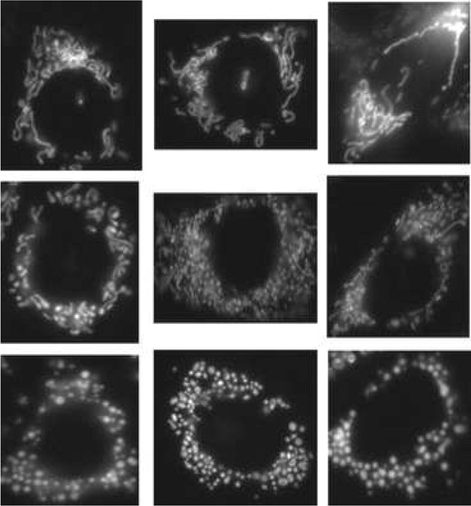
Example cell images show different fragmentation stages of mitochondria, tagged with a fluorescent dye. Images at the bottom row are cells with the completely fragmented mitochondria, at the top row are those without fragmentation, those in the middle are partially fragmented. From (Lin et al., 2010)
The challenge is to quantify and rank partial fragmentation as shown in the middle row. (Peng et al., 2011) concluded that z-LEHD was more effective than z-IETD in rescuing mitochondria from squamocin-induced fragmentation. This conclusion was used as the ground truth to assess the prediction accuracy of different methods later and images treated by squamocin and control were used as extreme cases.
Our database contains 257 images of cells treated with squamocin, 239 with z-IETD, 262 with z-LEHD and 238 control. We applied a feature extraction method to extract 135 features from each cell image to form the feature vector to represent each cell. This feature extraction method is the same as the one that was used to extract strong detectors from cell images to determine protein subcellular localization as described by Lin et al. (2007). Strong detectors include general purpose features derived from image transformations, such as Haralick texture features and geometric features of the objects extracted from the input image. These features have been shown to be useful in problems like recognizing fluorescent patterns of subcelluar organelles in protein subcellular localization (Huang and Murphy, 2004).
3 RESULTS
3.1 Formal Analysis of FABS-![graphic]()
as a solution to this problem. The drug ranking problem can be considered as a regression problem, where given a multi-dimensional observation vi=X∈ℜd, we assume that a quantity Y∈[−1, +1] is associated with X as our target metric of X. A solution of this regression problem is to learn a regression model from examples that compute Y given X. With the metric quantity Y, given two treatments a and b with population distributions  a and b, respectively, if
However, it is usually infeasible to manually assign score Y for a sufficient number of training examples consistently. Instead, FABS- simplifies the problem as a bipartition problem. In our bipartition scheme, our model will assign Yc=1 to a given X if Y≥0 and Yc=−1 otherwise, and then use empirical population mean as the estimated population mean of Y. In a drug screening application, this quantity will be used to rank the effectiveness of a treatment.
 compares the expectation of Yc to determine which treatment is more effective.
 be the estimation of Yc. Then
 , which is interesting because we can infer the expected difference between regression (equation 1) and bipartition (equation 2).
 . We have
The result above implies that when we have a weak classifier ε→0.5,  and
and  . That is, regardless of the population, random guessing will not give any distinction between any populations and provide no discerning power. In contrast, when we have a perfect classifier with ε→0,
  , which is to scale the true probability of Y≥0 for the population to [−1, 1], perfectly matching our desire. Consequently, given an accurate bipartition algorithm, FABS- can reasonably approximate effectiveness of drugs without exact scores the effectiveness.
3.2 Performance of ranking
We compared the performance of FABS-NC′ with four other baselines that has been used in HCS—center ranking PCA ranking and graph transition energy method (GTEM) (Lin et al., 2010). Center ranking first finds the center, which can be the mean, the median or any other measure of the center, of all feature vectors associated with a particular drug or an extreme case, then calculate the distance, such as Euclidean distance, between all pairs of centers. The ranking of the drugs are performed by ordering the drugs according to the centers of the closest to the farthest from the center of the desired extreme case (such as the completely fragmented state for toxicity criterion). PCA ranking is similar to center ranking, except it first projects the feature vectors onto the first few important principal components, then performs center ranking. GTEM (Lin et al., 2010) is also a graph-based approach. GTEM defines graph transition energy as the distance metric and utilizes a spectral graph theoretic regularization to transform the feature space so that extreme cases will be separated widely before ranks populations of cells under different treatments.
In addition to use NC′ [solved with Hochbaum's PseudoFlow algorithm, HPF, the implementation of which is obtained from (Chandran and Hochbaum, 2009; Hochbaum, 2008, 2010a)] as our bipartition algorithm in the FABS framework, we also tested other bipartition procedures. One classical technique is the SVM (Burges, 1998; Cristianini and Shawe-Taylor, 2000). When using SVM for FABS, we satisfy Requirement 1 by setting training data as the positive and negative controls: all R1 points are in S and all R2 points are in  . To see the performance of this particular implementation of (FABS-SVM), the kernel used is radial basis function and the parameters are the following: C value is 104 and the kernel parameter is 1. The implementation package used is LIBSVM (Chang and Lin, 2011).
Another approach, often used in image segmentation is based on finding the Fielder eigenvector of the graph (referred to as the spectral technique) as a heuristic solution for the normalized cut problem (Shi and Malik, 2000). The spectral technique however is unsupervised, and thus does not satisfy Requirement 1. To resolve this issue, we modified the weights of the graph to ensure that Requirement 1 is satisfied. The implementation package used is Normalized Cuts Segmentation Code, Timothee Cour (2004). However, its performance was much worse than all other methods and was removed from the results.
The comparative study that we performed used the median for all center measures and Euclidean distance for all distance measures. The edge weights between two feature vectors vi and vj increase or decrease in the opposite direction with respect to the distance between them and is quantified by wij=e−||vi−vj||2+ϵ, for 0<ε≪1.
Prior to feeding the input feature vectors extracted from the images into FABS-, we first pre-process these vectors to transform them from a high-dimension space to a space of fewer dimensions. In this process, the data are reduced to fewer dimensions, and we only preserve the dimensions that are of the most significance to our experiment. The dimension reduction is performed by using PCA and the number of principal components used is determined by adding the largest number of most significant principal components that explain up to 80% of the total variation in the dataset considered. We also tested whether applying GTEMs feature transformation step as a preprocessing step before applying FABS-NC′ may improve the performance.
To guarantee statistical validity of our comparison, we subsampled the available cell images from the entire database, i.e. we drew samples with replacement for certain percentage from the database to test methods. The subsampling percentages 30, 60, 70 and 80 tried for drug images (501 images). For each fixed drug percentage, we changed percentages of labeled controls by increasing from 10% to 100% to see the effects of the number of labeled controls on the final prediction accuracy of the ranking (495 images in total). The subsampling trials are performed 1000 times for each combination. The prediction accuracy of any ranking method is the fraction of correctly ranked trials—this can be determined, since we have the ground truth—out of the grand total of 1000 trials.
Figures 3 and 4 graphically summarize the results in the experiment. Each graph shown is for 30, 60, 70 or 80% fixed drug percentage (testing percentage). The x-axis is the percentage of labeled controls used, whereas y-axis displays the average prediction accuracy over 1000 trials described in Section 3.2.
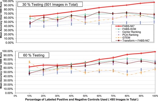
The accuracy comparison among different ranking methods. The vertical bars in the graph are 95% confidence intervals. The testing percentages used are: 30 and 60%
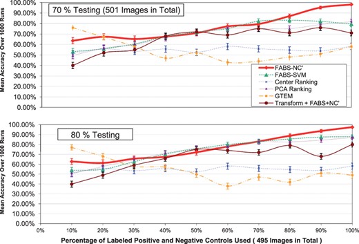
(Continued) the testing percentages used are: 70 and 80%
Each curve in the graphs indicates a particular ranking method—they include FABS-NC′, FABS-SVM, Center ranking, PCA ranking, GTEM. The results of FABS-Spectral is poor with our particular implementation and from the figures. The vertical lines in Figures 3 and 4 are 95% confidence intervals for the accuracy of each ranking method.
For all testing percentages, the prediction accuracy of FABS-NC′ steadily increases as more labeled controls become available, especially when more images are tested (70 and 80%)—the slope increases then levels off from the left to the right. The overall accuracy is nearly 98% for all graphs at the end of the x-axis, indicating that the method is highly accurate with as little as 500 labeled controls. It is also robust considering that the trend of prediction curve remains the same for different testing percentages.
Moreover, we can see that FABS-NC′ has an advantage over other ranking methods for this particular mitochondria dataset. Its curve is often above all other methods, except for 10 labeled controls; testing percentage 70%: 70% labeled controls; and testing percentage 80%: 10% and interval 40–50%. Notice that for the low number of testing (30%), FABS-NC′ outperforms all other methods—when using all labeled controls for ranking, it is over half more accurate than the next best algorithm.
Overall, FABS-SVM also performs well, although sometimes trailing behind FABS-NC′ by a large margin. PCA ranking performs poorly when testing images are few (30%). Center ranking is generally of low quality, giving small accuracy for all testing percentages. Notice, however, GTEM gives the best results when the number of labeled controls is very low (10%), indicating its usefulness when training data are few—neverthless, its advantage dimishes as more labeled training cases becomes available, producing inaccurate rankings comparing to FABS. The results show that applying the feature transformation step of GTEM as a pre-processing step of FABS-NC′ performs better than GTEM but not as well and as stable as FABS-NC′.
The experimental results suggest that, overall, FABS with NC′ implementation is the best ranking method among all for this particular mitochondria database. Remarkably, FABS-NC′ generalizes better than any other methods as more training and test examples become available.
3.3 Significance
Table 1 displays the significance score −log P between different pairs of drugs for FABS-NC′ and FABS-SVM implementations when we sub-sampled 30% of the labeled controls and 30% of drug treatment results. An infinity score (∞) is obtained when P is very close to zero, indicating that the distance between the two corresponding drugs is very large. The results show that FABS-NC′ is more discriminant then FAB-SVM because the significance scores for FABS-NC′ are larger than those for FABS-SVM.
Matrices of GDM between different pairs of drugs for different implementations of FABS-SVM and FABS-NC′
| FABS-SVM | squamocin | Z-IETD | Z-LEHD |
|---|---|---|---|
| squamocin | 0 | ∞ | ∞ |
| Z-IETD | ∞ | 0 | 3.43 |
| Z-LEHD | ∞ | 3.43 | 0 |
| FABS-NC′ | |||
| squamocin | 0 | ∞ | ∞ |
| Z-IETD | ∞ | 0 | 4.36 |
| Z-LEHD | ∞ | 4.36 | 0 |
| FABS-SVM | squamocin | Z-IETD | Z-LEHD |
|---|---|---|---|
| squamocin | 0 | ∞ | ∞ |
| Z-IETD | ∞ | 0 | 3.43 |
| Z-LEHD | ∞ | 3.43 | 0 |
| FABS-NC′ | |||
| squamocin | 0 | ∞ | ∞ |
| Z-IETD | ∞ | 0 | 4.36 |
| Z-LEHD | ∞ | 4.36 | 0 |
We also performed a Monte Carlo simulation to test whether the observed difference of the FABS-NC′ scores of 30% of Z-IETD and Z-LEHD data using 80% of control data for training is significant against pairs of null data sets sampled from the same drug treatment populations. In 1000 random resamplings, no difference of the scores of the null data set pairs is higher than the observed score, yielding a close to zero P-value.
3.4 Comparison of running time
In this section, we compare the running times of three FABS- procedures, where here, as mentioned in previous sections, is one of bipartition algorithms including NC′ (Hochbaum, 2010b), SVM (Cristianini and Shawe-Taylor, 2000) and Spectral (Shi and Malik, 2000), among themselves and against PCA ranking, Center ranking and GTEM. The specification of the computer environment for this comparison is a Windows computer with 2.4GHz Intel(R) Core(TM)2 Duo CPU 2.40 GHz and 2 GB memory.
Figures 5 and 6 display running times of various methods, excluding the times for subsampling—which have a median of 0.01 second, maximum of 0.02 second and minimum of 0.006 second—for different testing percentages: x-axis increases with the number of positive controls and negative controls used, representing more and more training data becoming available, while y-axis is the running time. The six curves in the figures are the different methods including various implementations of FABS-—notice that FABS-NC′ is represented by the thickest curve. There are 501 testing data: 265 Z-IETD and 291 Z-LEHD.
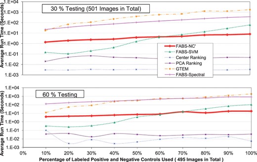
The running time comparison among different methods. The testing percentages used are: 30 and 60%

(Continued) the testing percentages used are: 70 and 80%
From the figures, among FABS-, we can observe that for all testing percentages considered, FABS-Spectral takes the most running time, lagging behind both FABS-NC′ and FABS-SVM by large margins. For FABS-NC′, the running time steadily lengthens as the number of positive and negative controls increases, however, not as dramatic as FABS-SVM, whose running time, shorter than these of other procedures initially, grows exponentially—in one case (testing percentage 70%), running 100% of positive and negative controls requires around 1000 times more seconds than running 10% of positive and negative controls. This is to compare with FABS-NC′: for the same testing percentage, using all positve and negative controls only requires twice as much running time than that of using only 10%—10 corresponds to around 50 controls in total, a relative small number of images that can be obtained through HCS. This observation, combined with the results from Section 3.2, indicates that even though FABS-SVM has the initial advantage for running time, this is off-set by the initial more accurate results produced by FABS-NC′. Moreover, it appears that FABS−NC′ scales much better with increasing input data than FABS-SVM. Looking at the other methods besides FABS-, we can observe that GTEM takes relatively long time on the par with FABS-Spectral—this is in contrast with PCA ranking and center ranking whose running times are the lowest among all methods: this result is expected, since FABS- use PCA for pre-processing (i.e. doing PCA is already added as a part of computational costs), therefore FABS- can only take longer time than PCA ranking. However, from Section 3.2, it is clear that this extra computational costs bring significant improvements in accuracy, which combined with scalability of FABS-NC′, makes FABS-NC′, overall, an attractive candidate for ranking this database.
4 DISCUSSION
In this article, we describe a new drug ranking framework called FABS. It is graph based, producing a single scalar score for each drug for ranking. The formulation and solution sidesteps many pitfalls of other traditional methods. The article also reports FABS-NC′ semi-supervised implementation and its comparative study. Not only is this implementation better than four other considered methods, it also outperforms FABS-SVM and FABS-spectral implementations on a mitochondria databases. This preliminary result suggests that FABS-NC′ is good for ranking toxicity of drugs targeting mitochondria for a specific database.
There are some advantages of our measure. First, FABS is one-dimensional, that is, a single scalar, giving an unambiguous way to rank drugs. Its computation considers all samples of each drug and uses a fraction as the final score. This diminishes the effect of outliers and noise, because, if the number of images is large for each drug, as in the case of HCS, outliers, which are few in number, can not influence the result—a fraction, in a significant way. This similarly is the reason for noise reduction. More importantly, our measure FABS-NC′ is acquired through a combinatorial algorithm, which is efficient. This is essential since the number of cells observed in a HCS is large and the applicability of any metric learning algorithm is greatly reduced if it cannot process them sufficiently fast. The last noteworthy advantage of our framework is that the training data for the semi-supervised formulation are the positive and negative controls, which are easily recognizable and obtained without time-consuming annotation, sidestepping the limitation of training sample size of many metric learning algorithms.
Our future work includes to investigate whether the introduction of node weights, in our construction of the graph in Step 2 of Algorithm 1 will benefit the prediction results. This is especially relevant because of a recent development for solving generalized version of NC′ utilizing node weights (Hochbaum, 2010c). Moreover, we could also expand our FABS application into other criteria and situations for determining the ranking of the drugs and test on more databases to see the effectiveness of our method as they become available.
ACKNOWLEDGMENTS
We wish to thank Professor Chung-Chi Lin and his team at the National Yang-Ming University, Taiwan for providing us the image database used in our experiments.
Funding: National Science Foundation awards (No. DMI-0620677, CMMI-1200592 and CBET-0736232 to D.8.H. partial). The National Heart, Lung, and Blood Institute award (1UH2HL108780-01 to C.N.H. partial)
REFERENCES
Author notes
†The author wish it to be known that, in their opinion, the first two authors should be regarded as the joint first Authors.

