TSSi—an R package for transcription start site identification from 5′ mRNA tag data Free

Abstract

1 INTRODUCTION

High-throughput sequencing has become an essential experimental approach to investigate genomes and transcriptional processes. The core of most applications is a peak finding algorithm which is required to identify regions of interest. These algorithms are designed application specifically because the requirements depend on characteristics of the measurements as well as on the questions of interest. While cDNA sequencing (RNA-seq) using random priming and/or fragmentation of cDNA will result in a shallow distribution of reads typically biased toward the 3′ end, approaches like CAP-capture enrich 5′ ends of mRNAs and result in distinguishable peaks around the transcription start site(s) (TSSs). Similar methods can also be applied to specifically target 3′ ends of mRNAs. The resolution and utility of the multitude of end-tagging methods have been tremendously increased in recent years by the application of next-generation sequencing technologies which allow 5′ or 3′ digital gene expression at genome scale (Hoskins et al., 2011). When applied to sequencing of DNA fragments isolated by immunoprecipitation (ChIP-seq) broad and almost unimodal densities without gaps are obtained around a target position which, depending on the protein used for immunoprecipitation, usually represents a transcription factor binding site or provides insight into chromatin structure. For such applications, several approaches have been proposed although benchmark problems show that these algorithms still work insufficiently in some cases (references are provided in the Supplementary Material).

Predicting the location of TSSs is complicated by the possible existence of an unknown number of multiple, alternative TSSs. Furthermore, the transcription of many genes in eukaryotic genomes is initiated at not well-defined sharp or peaked sites, but in more fuzzily defined, broad transcription start regions (see references in the Supplementary Material). In addition, as illustrated in Figure 1, the measurements typically contain background reads, i.e. false positives not originating from real TSSs. Therefore, only the counts which are significantly larger than an expected number of background reads are intended to be predicted as TSSs. The 5′ end tag data used as a test set for our study (see Section 2) comprises reads mapping to 211 669 genomic positions. This vastly exceeds the expected number of TSSs, indicating the existence of reads not originating from real TSSs. Such reads cluster to certain genomic positions, i.e. the level of background noise seems to be proportional to proximate measurements yielding false positive reads preferably in regions of transcriptional activity. It is yet unclear, whether these are artifacts introduced from the experimental procedure or whether there is a biological meaning to this noise. As currently there is no error model available describing such noise, an heuristic approach is introduced for an automated and flexible prediction of TSSs in the following.

Fig. 1.

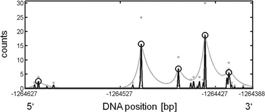
An example illustrating the results of the TSSi analysis for 5′ tag data. The horizontal axis is the genomic position of the transcribed DNA sequence, in this example on scaffold 1. Negative numbers on this axis indicate the anti-sense strand, i.e. transcription in the plot occurs from left to right. The raw reads at positions of the respective 5′ ends of the template DNA sequences are plotted as gray dots. The measurements processed by the regularization procedure are plotted as black lines and the predicted TSSs are depicted as black circles. The gray line indicates the contamination threshold level. For this illustration, λ₁=1, λ₂=0.1, τ_5′=5 and τ_3′=10 have been chosen

Open in new tabDownload slide

2 METHODOLOGY

As input, our method uses the number y_i of sequenced transcripts as well as the genomic position i of the 5′ end of the mapped DNA sequences given by the chromosome/scaffold, the strand and the genomic position. As an example, we have analyzed 76 nt Illumina CAP-capture (5′ tag) data generated from protonema tissue of the moss Physcomitrella patens following the protocol of Maruyama and Sugano (1994). As a preprocessing of such data for use with TSSi reads need to be mapped to the reference genome to acquire read counts and position information. For computational efficiency, the analysis is iteratively performed on all segments with transcriptional activity. Further preprocessing, e.g. restriction to upstream regions of annotated genes, is optional (see Supplementary Material for details).

The first step in our analysis is a preprocessing procedure which reduces the noise by shrinking the counts toward zero. This step is intended to eliminate false positive counts as well as making further analyses more robust by reducing the impact of large counts. Such a shrinkage or regularization procedure constitutes a well-established strategy in statistics to make predictions conservative, i.e. to reduce the number of false positive predictions (Tibshirani, 1996).

Two regularization parameters λ₁ and λ₂ are used for the objective function

(1)

to be minimized to estimate the transcription level in a regularized manner. Here, N denotes the number of genomic positions, the vector represents the true transcription level, is the vector of measurements, i.e. the reads, and indicates the estimated level of transcription. The log-likelihood is given by the product of the probabilities of the counts y_i which is assumed as a Poisson distribution

(2)

with expectations x_i by default. The current implementation also allows user-specific probability distributions, e.g. a negative binomial distribution. For λ₁>0, counts unequal to zero are penalized by the second term in (1) to obtain conservative estimates of the transcription levels with a preferably small number of components, i.e. genomic positions, unequal to zero. The larger λ₁, the more conservative is the identification procedure. To enhance the shrinkage of isolated counts in comparison to counts in regions of strong transcriptional activity, the information of consecutive genomic positions in the measurements is regarded by the third term in (1), i.e. by evaluating differences |x_i−x_i−1| between adjacent count estimates. Without regularization, i.e. for λ₁=λ₂=0, is the maximum-likelihood estimator of the expectation of the count distribution.

After the regularization procedure, an iterative algorithm is applied for each analyzed genomic region, typically the upstream region of a translation start, e.g. up to the length of a typical or the longest known 5′ untranslated region in that organism, to identify the TSSs. The expected number of false positive/background counts x^FP is initialized with a default value of ∑_i=1^Ny_i/N which is given by the read frequency in the whole dataset. The position with the largest counts exceeding x^FP is identified as a TSS if the expected transcription level is at least one read exceeding the expected number of false positive reads, i.e. ⁠. The transcription levels for all TSSs t are calculated by adding all counts x_i to their nearest neighbor TSS. Then, the expected number of background reads is updated by convolution

(3)

with exponential kernels. The decay rates τ_5′ in 5′ direction and τ_3′ toward the 3' end can be chosen independently to account for the fact that false positive counts are preferably found in 3′ direction of a TSS. This procedure is iterated as long as the set of TSSs increases.

For the exemplary region displayed in Figure 1, the raw counts y_i are plotted as gray dots, the regularized count estimates are plotted as black lines, and the predicted TSSs are labeled by black circles. The exponentially decaying expected rates of background counts x^FP are plotted as gray lines. In the Supplementary Material, the effects of changing the parameters λ₁, λ₂, τ_5′ and τ_3′ are illustrated.

3 CONCLUSIONS

An important application of high-throughput sequencing is the identification of TSSs. In this application note, the R package TSSi is introduced for the prediction of TSSs based on the mapped 5′ ends of mRNAs. As an optional preprocessing step, the transcription level is estimated by regularization to make the TSS predictions conservative.

Unless user-defined distributions are applied, a Poisson distribution for the counts and an exponentially decaying expected number of background reads proximate to TSSs are assumed. Since our implementation allows a flexible, project-specific adaptation, the method could also be valuable for peak finding problems in other applications.

The presented method does not use any prior information about potential TSSs, e.g. provided by annotation like transcription factor binding sites. Extending the method concerning such information could be a future task.

ACKNOWLEDGEMENTS

The authors acknowledge German Federal Ministry of Education and Research (BMBF) and German Research Foundation (DFG).

Funding: German Federal Ministry of Education and Research (BMBF) [0315766-VirtualLiver] and [0313921-FRISYS]; German Research Foundation (DFG) [RE 837/10-2].

Conflict of Interest: none declared.

REFERENCES

Author notes