optiCall: a robust genotype-calling algorithm for rare, low-frequency and common variants Open Access

Abstract

1 INTRODUCTION

Burgeoning whole-genome and whole-exome sequencing projects are likely to require large-scale microarray-based follow-up studies. Already, custom arrays, such as Metabochip and Immunochip, utilize SNPs identified through population-based sequencing efforts such as 1000 genomes to better survey loci known to underpin variation across related phenotypes (Trynka et al., 2011). Typically, the allelic probes on these custom arrays have undergone less stringent quality control (QC) compared to those that make it onto mass-produced GWAS arrays. This drop in probe quality, in addition to a greater focus on low-frequency and rare variants (those with minor allele frequencies 0.5–5% and <0.5%, respectively; The 1000 Genomes Project Consortium, 2010) presents many problems for existing genotype-calling algorithms.

Genotype-calling algorithms use normalized measures of DNA binding to allele specific probes to ascertain the genotype of an individual at a given SNP. As an example, a wild-type homozygous genotype at a particular SNP would have a high intensity value for the wild-type allelic probe, and little or no intensity for the alternative allelic probe. A heterozygous sample would have intermediate intensities for both probes. Existing callers vary in both the statistical models they apply, and how they utilize the intensity data across individuals and SNPs.

Illumina's proprietary genotype-calling software, GenCall, uses a custom clustering algorithm that encompasses several biological heuristics to determine genotypes from intensity clouds obtained by gathering all individuals at a single SNP. If less than three well-defined genotype clusters are observed, GenCall uses a neural network model to estimate the location and shape of the undefined clusters. GenCall is designed to work on Illumina arrays and, being based on a pretrained neural network, its performance on a new dataset is dependent on how close the new data matches the data used to train the network.

Another commonly used genotype-calling algorithm, Illuminus (Teo et al., 2007), also designed for Illumina arrays, again clusters intensity data across samples on a per SNP basis, using an unsupervised clustering method based on a mixture model of Student's t-distributions. This unsupervised approach removes the need for a called training set. However, low-frequency SNPs and/or small sample sizes can result in poorly defined clusters and inaccurate genotype calls due to the small number of rare allele observations. Giannoulatou et al. (2008) discovered within-sample intensity data also tended to cluster into three distinct genotype groups. On the basis of this observation, they created GenoSNP, a within-sample genotype-calling algorithm. Clustering within sample can be advantageous for rare variants and small sample sizes, as three well-defined clusters are always observed. A drawback of the approach is that intensity variation between SNPs is not accounted for, resulting in inaccurate genotype calls for SNPs where intensity clusters are shifted from their expected positions.

We have developed optiCall, a novel genotype-calling algorithm that uses both within and across sample intensity data to accurately ascertain genotypes from across the minor allele frequency spectrum. In the following sections, we describe optiCall and compare its output to that from existing algorithms using 4537 samples from the 1958 British Birth Cohort (Power and Elliott, 2006) genotyped on the Immunochip, an Illumina iSelect HD custom array (Cortes and Brown, 2011).

2 METHODS

2.1 Data

Illumina uses a six degree of freedom affine transformation to normalize data for channel-dependent background and global intensity differences. The data input to the algorithm have a normalized intensity point x=(x₍₁₎,x₍₂₎) for each sample and SNP on the array, indicating the binding strength of the sample's DNA to the probes for each of the two alleles being interrogated at the SNP.

2.2 Creating the within and across sample prior

optiCall first takes a random subset S of intensity values from the data (by default |S| is the minimum of 50 000 and the size of the dataset). Every element in S is a (x₍₁₎, x₍₂₎) normalized intensity point for a random sample at a random SNP. This subset, of both within and across sample intensities, is used to create a data-derived prior distribution on the intensity space, defining regions of high probability for each genotype class. A four-class mixture model of Student's t-distributions is used to model the data, with a class corresponding to each genotype and one class to catch outliers of unknown genotype. So for each element x_j in S, there is a latent genotype variable g_j∈{1, 2, 3, 4} and the joint probability density function (pdf) of (x_j, g_j) under the mixture model is given by

(1)

and for the entire subset S×G={(x_j, g_j):x_j∈S}:

(2)

where π_i are the class probabilities, such that the π_i sum to 1, I is the indicator function, and each p_i is the pdf of a Student's t-distribution with location parameter μ_i, covariance Σ_i and scale parameter v_i, for simplicity all represented by the parameter vector θ.

The model is fitted to the data by inferring values for the π_i, μ_i, Σ_i to maximize the likelihood of the data by an expectation maximization (EM) procedure (Dempster et al., 1977). The parameters μ_i, Σ_i are fixed for the unknown class [by default (0,0) and 100×I₂, where I₂ is the 2 × 2 identity matrix] so that the probability density is even over parameter space, and outliers are assigned unknown. The v_i for all classes are also fixed at 1.

When performing inference, initial values for the μ_i, Σ_i of the genotype classes are obtained from a run of the k means ++ clustering algorithm for k equal to three (Arthur and Vassilvitskii, 2007), and all the π_i are each set to 0.25. Using the EM algorithm, the initial parameter values are altered so that they maximize the log-likelihood of the data. The unknown class is treated like the genotype classes during inference, except for its mean and covariance parameters remaining fixed. The EM algorithm obtains a (possibly local) maximum for the log-likelihood by alternating between an expectation (E) step, and a maximization (M) step. For the E-step, the expected value of the log likelihood is calculated, with respect to the latent variable given the current values of the parameters. Next the M-step finds the parameters to maximize this expected log-likelihood, the parameter values are updated, and the algorithm moves to the next iteration of EM steps.

Equation (2) is the expression for the likelihood of the data, and the log-likelihood expression is shown in (3).

(3)

with the latent variable z_ij being the value of I(g_j=i) The z_ij are updated on the E-step, being set to the posterior probabilities of class membership—given the current estimates for θ, and the θ are set on the M-step. The derivation of the latent variable and parameter update equations of the EM algorithm for a mixture of t-distributions can be found in McLachlan and Peel (2000). The EM algorithm is halted after 30 iterations, but stops early if genotype calls are unchanged for more than three consecutive iterations, and final parameter values are subsequently taken.

The across sample and SNP clustering happens only once, and the resulting mixture model provides prior information in subsequent per SNP, across sample, clustering steps.

2.3 Genotype calls across samples with prior information across SNPs

optiCall next goes through the intensity data SNP-wise, gathering all sample intensities at a SNP, and clustering with another mixture model of Student's t-distributions. The mixture model again has four classes, one for each genotype, and an additional one for outliers. However, instead of maximizing the likelihood, a prior is incorporated on the model parameter vector θ, based on the clustering of S, and the posterior is maximized to get the Maximum A-Posteriori estimate for the parameters θ. Thus, ignoring the term p(S×G) which is unaffected by the choice of θ, optiCall aims to find the θ maximizing:

(4)

which in our case is shown in (5):

(5)

For the three genotype classes (i=1, 2, 3), we put a Normal–Wishart prior distribution on the location and precision matrix of each genotype's t-distribution:

(6)

where α_i, β_i, γ_i, S_i are hyperparameters assigned values based on the clustering step from (2.2). The α_i are set to the optimal μ_i obtained from the results of the clustering in (2.2); similarly the S_i are set to the inverse of the optimal Σ_i. The β_i are set to 1, and the γ_i to 100. For the unknown class (i=4), the μ_i, Σ_i are fixed as in (2.2), meaning the prior distribution p₄ (μ₄, Σ₄) essentially assigns all its probability density at these values of μ_i, Σ_i. The v_i similarly are set to 1 for all classes apart from the heterozygous class, which is set to 1.3.

To infer the values of the π_i, μ_i, Σ_i we use a modified EM procedure, with starting points for the π_i set to their optimum values found in (2.2). Initial values for μ_i and Σ_i are also their optimal equivalents from (2.2) but multiplied (element-wise) by the scaling factors:

to account for SNP specific intensity shifts. and are the mean and SD of the intensity data of the current SNP, μ_het is the optimal μ_i of the heterozygous class from (2.2), is the SD of the random subset S from (2.2), and bracketed subscripts show the allele (1 or 2) over which the mean or SD is calculated, for points (x₍₁₎,x₍₂₎). The modification to the EM procedure occurs at the E-step when calculating the expected value of z_ij. If the maximum genotype posterior probability for an intensity point p(g_j=i|x_j) is above 0.9, according to the model inferred in (2.2), the expected value for z_ij is calculated using these genotype posteriors, instead of the values of π_i in the current clustering. This way, points with highly confident genotype posteriors by the model in (2.2), but possibly forming a sparse cluster, can still guide the current clustering (Fig. 1b). The EM algorithm runs for 15 iterations but stops early if genotype calls are unchanged for more than three consecutive iterations.

Fig. 1.

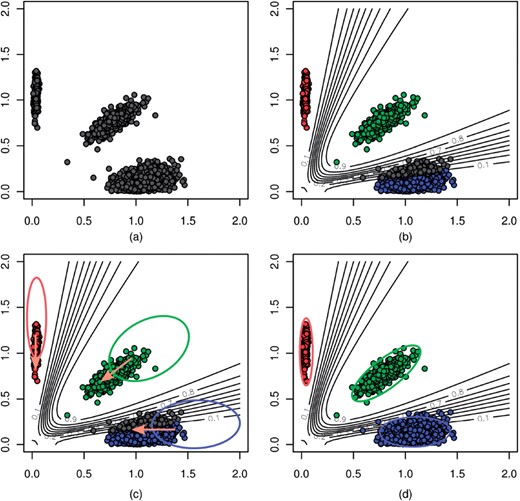
Calling a SNP with optiCall. In (a) intensity data is taken from all samples at the SNP. Then, using a data-derived (within and across sample) prior, and adjusting class membership probabilities based on the prior in an EM procedure (b and c), a mixture model of Student's t-distributions is fitted to the data (d)

Open in new tabDownload slide

Once the optimal parameter values are inferred, genotype posterior probabilities for a data point from the model are calculated according to (7). The μ_i, Σ_i and v_i are from the results of the current SNP-wise clustering, while π_i^′ are the genotype posterior probabilities for x_j calculated using v_i and optimum values for π_i, μ_i, Σ_i from (2.2). Using π_i^′ in this way helps in clustering rare variants, which may be only a few points, but falling in a high probability region according to (2.2). Genotypes are called for any points with a class posterior probability of at least 0.7 (by default), with those falling below this threshold called unknown.

(7)

2.4 Measuring clustering quality and reclassifying poorly clustered SNPs

optiCall uses deviation from Hardy–Weinberg equilibrium (HWE) as an indicator of clustering quality. A χ² test is used to test HWE unless sample size is small (<50 expected counts of any genotype, assuming HWE or allele counts of <100 for either allele), in which case an exact test is used (Wigginton et al., 2005). SNPs with a HWE P-value less than a given threshold (P<5×10⁻¹⁵ by default) are deemed to be poorly called. optiCall attempts to improve the genotype calls at these SNPs by again running a Student's t-based mixture model, but this time omitting the SNP and sample-wise prior. This rescue step is primarily implemented to give better genotype calls at SNPs where the genotype intensity clouds lie outside of the expected regions defined by the within and across sample prior. The statistical model is as described in (1) and (2), with the intensity values first transformed according to (8), to improve calling of SNPs with shifted intensities (Teo et al., 2007).

(8)

Inference is as in (2.2), by the EM algorithm. The ν_i are fixed at 1 for all classes except the heterozygous class, which is fixed at 1.3. The values of μ_i, Σ_i for the unknown class are fixed with identical values to (2.2).

All four classes have initial class probabilities set to 0.25, and for the three genotype classes initial covariance matrices are set to (2c/N)×I₂ with c the cost (Arthur and Vassilvitskii, 2007) of a k means ++ clustering on the data, and N the number of intensity points. The transformation of intensities has accounted for shifts, and so location parameters of the two homozygous classes can be initialized to the extremes of y₍₁₎, and the heterozygous class will then fall somewhere in between, thus the μ_i are initialized to

(9)

where the min/max are taken over a filtered version of the intensity data, with the lowest 1% of untransformed intensity values in the x₍₁₎ direction and lowest one percent in the x₍₂₎ direction removed. is the mean of the y_j over the second axis, and k is a shift parameter for the location of the heterozygous class, that takes one of three values, 0.45, 0.5 or 0.55, resulting in three sets of initial values dependent on the value of k. For each set of starting values, the EM algorithm is run until genotype calls are concordant for two consecutive iterations, and the optimal parameters are chosen to be the final values with the highest likelihood.

Genotype calls are made using genotype posterior probabilities [using the π_i inferred from this step unlike (2.3)] with a 0.7 call threshold. By default, SNPs that fail the HWE test subsequent to this step have all genotypes called unknown.

In our experiments, we have found the occurrence of the rescue step, and the subsequent chances of a successful rescue, to vary with the quality of the dataset. On a number of Immunochip datasets, rescue steps tended to occur on between 3 and 10% of SNPs, with 30–50% being successful.

3 RESULTS

To test the performance of optiCall, and compare it to existing algorithms, we used data from 4537 individuals from the 1958 British Birth Cohort who were genotyped using the Immunochip, an Illumina iSelect HD custom array designed for deep replication of autoimmune disease genome-wide association study results and fine-mapping within 184 known autoimmune disease loci (Trynka et al., 2011). Genotypes were called at 192 402 SNPs using optiCall, GenCall, Illuminus and GenoSNP. Default parameters were used when running each of the algorithms.

The genotype data from each algorithm underwent a simple QC protocol to reflect a typical association study. SNPs failed QC if they had a call rate <98% or HWE P<10⁻⁵. Table 1 shows the QC results for each caller across the dataset.

Calls from Illuminus and GenoSNP produce the most discordant results at QC (with 5157 and 8815 unique QC passes and fails, respectively) whereas GenCall and optiCall appear to have more overlapping QC outcomes with other callers.

3.1 SNPs passing/failing QC

In an association study, if many SNPs fail QC because of poor genotype calling, potential casual variants may be missed. However, too many calls incorrectly passing QC would result in increased false-positive associations, and more overheads in subsequent follow-up and replication.

To assess clustering quality and accuracy, 600 unique QC pass SNPs and 600 unique QC fail SNPs were selected at random and manually called using a modified version of Evoker (Morris et al., 2010). All manual calling was carried out blind to genotype calls from any of the algorithms. The 1200 SNPs were split into four subsets, each manually called by a different person. Any SNPs deemed difficult to call were blind re-called by all four human callers, and the consensus genotypes were taken forward. Manually called genotypes were then compared to those from each of the genotype-calling algorithms, classifying SNPs passing QC for both the algorithm and manual call set as true-pass (TP) SNPs, and SNPs failing QC in the manual calls but passing QC for the given algorithm as false-pass (FP) calls. Similarly, SNPs failing QC for both the manual calls and the algorithm were classified as true-fail (TF) SNPs, while false-fail (FF) SNPs fail QC for the given algorithm only. Sensitivity and specificity were then calculated for each of the algorithms (Table 2).

For the sampled data optiCall yielded the highest sensitivity, but with a lower specificity compared to GenCall and GenoSNP. GenoSNP's sensitivity was significantly lower than its counterparts, as was Illuminus' specificity. Anecdotally, many of GenoSNP's FFs occurred at SNPs where intensity data were shifted from the expected positions, a drawback of the within-individual clustering approach.

R-squared values (Pearson correlation coefficient where genotypes are placed on a 0, 1, 2 scale and unknown genotypes are assigned the numerical mean genotype) to the manual calls for TP SNPs were high across all three callers (0.995 for Illuminus, 0.983 for GenoSNP, 0.990 for GenCall and optiCall), suggesting that SNPs passing QC are called accurately by all algorithms.

3.2 Missed rare variants

Genetic association studies are increasingly focusing on identifying rare variation underlying disease susceptibility (Manolio et al., 2009). To investigate how well each of the algorithms captures such variants, we randomly selected 600 SNPs that were monomorphic in one algorithm but had a minor allele frequency between 4×10⁻⁴ and 0.01 in at least another two. Manual calling was carried out as described in Section 3.1. Of the 600 manually called SNPs, Illuminus misclassified 354 rare SNPs as monomorphic, while GenoSNP, GenCall and optiCall misclassified only 3, 13 and 1, respectively. This high number of misclassified rare variants is a direct consequence of Illuminus' within SNP, across sample, approach to genotype calling.

3.3 Comparison to manually called genotypes across chromosome 21

To assess how well each of the algorithms performed across a random selection of SNPs on the Immunochip, we manually called the 1868 SNPs on chromosome 21 using the same procedure as outlined in Section 3.1. Again, SNPs with a call rate <0.98 and/or HWE P<10⁻⁵ were deemed to have failed QC. QC results from the genotype-calling algorithms were then compared to those from the manually called genotypes. Although less pronounced than previous comparisons, which specifically focused on SNPs at which the genotype-calling algorithms disagreed, the same general trends were observed (Table 3). Of the 1810 SNPs passing QC in the manually called data, optiCall passed the most (1785 with a sensitivity of 0.99) and GenoSNP the least (1668 with a sensitivity of 0.92). GenCall and Illuminus lay in between (GenCall passing 1737 SNPs and Illuminus 1761, with sensitivities of 0.96 and 0.97, respectively). GenoSNP and optiCall did not misclassify any of the low-frequency SNPs as monomorphic, while GenCall misclassified just one and Illuminus misclassified 21. As expected, SNPs correctly passing QC and then correctly called polymorphic for each algorithm have highly concordant calls to the manual call set (r²>0.993 for all callers).

By combining the FF rate and the number of misclassified rare variants across each genotype-calling algorithm, the loss percentages over the 1868 SNPs of chromosome 21 are 3.87, 7.85, 4.09 and 1.38% for Illuminus, GenoSNP, GenCall and optiCall, respectively. Extending this result over the entire Immunochip, we estimate that 7440, 15 094, 7865 and 2657 ‘callable’ SNPs will be falsely removed from analysis using Illuminus, GenoSNP, GenCall and optiCall, respectively.

4 DISCUSSION

Complex disease genetic association studies are increasingly focusing on rare and low-frequency variants, either using off-the-shelf genome-wide products such as the Illumina HumanOmni5-Quad or mass-produced targeted custom arrays such as the Metabochip, Immunochip or Exomechip. To improve genotype calling for such arrays, we have developed a new algorithm, optiCall, which uses both within and across sample intensity data when calling genotypes. Considering both sets of information simultaneously means optiCall captures the rare and low-frequency variants some purely SNP-wise genotype-calling algorithms can miss, while remaining robust to genotype intensity clouds lying away from their expected positions. Given that the allelic probes on custom arrays have undergone less stringent QC compared to those that make it onto mass-produced genome-wide SNP arrays, the ability to correctly call such SNPs can greatly increase the number of SNPs passing QC (and thus increase power to detect association).

We have shown that, of the existing genotype-calling algorithms, optiCall has the highest sensitivity in terms of SNPs passing basic QC. This is significant because each SNP that is removed from a study due to poor genotype calling is potentially a missed association. Furthermore, with reduced linkage disequilibrium observed at rare and low-frequency SNPs (in comparison to common variants), it is less likely that an association to such a variant will be detected through additional tag SNPs. This increase in sensitivity does also yield a small decrease in specificity but, given that cluster plots of associated variants can be manually checked prior to embarking on replication studies, the consequences of this in terms of false-positive associations are likely minimal.

Unlike some existing genotype-calling algorithms, optiCall estimates the positions of the genotype classes using the given intensity data and does not require a training dataset or predefined cluster file. This removes genotype-calling errors that manifest through differences between the training dataset and that under study. As more studies attempt to jointly analyze data from different genotyping laboratories and across many different ethnicities, such errors have the possibility to not only reduce power but also to increase false-positive associations. When using optiCall, we recommend that divergent populations (such as African-Americans and white Europeans) be called separately so population specific within and across sample priors are used. Some existing calling-algorithms allow users to manually re-position the predefined clusters to better match discordant datasets whereas optiCall automates this potentially labor intensive procedure. Importantly, optiCall's use of both within and across sample intensity data ensures it is more robust to small sample sizes than mixture model-based algorithms that only use SNP-wise data. Recently, Li et al. (2012) published a genotype-calling algorithm for the Illumina platform, M³, that also uses both within and across sample information when making genotype calls. M³ runs a two-step calling process. The first step involves calling across sample, and then selecting a set of possibly poorly called SNPs (based on call rate and minor allele frequency) to call using across SNP information. optiCall differs from M³ in that it makes genotype calls using both within and across sample information simultaneously. M³ is written in Matlab, and we did not possess the necessary software to make a quantitative comparison.

A drawback of optiCall's genotype-calling approach is that it is very sensitive to intensity outliers (because these prevent the mixture models from fitting well). If no intensity outlier removal is performed prior to running optiCall, we recommend running optiCall's built in outlier removal. This process calculates the mean intensity difference x₍₁₎−x₍₂₎ over SNPs for each sample and those with a mean intensity difference more than 2 SD away from the mean are removed before genotype calling.

In summary, we have developed a new genotype-calling algorithm for Illumina arrays that uses both SNP-wise and sample-wise calling to more accurately ascertain genotypes at rare, low-frequency and common variants, even when genotype intensity clouds are shifted from their expected positions.

ACKNOWLEDGEMENTS

We wish to thank Luke Jostins and Andrew Morris for helpful comments on the algorithm and manuscript. We also thank Rob Andrews and Hannah Blackburn for providing genotype calls from Illuminus, GenoSNP and GenCall. We acknowledge the WTCCC2, 1958 British Cohort and the Immunochip consortium for access to samples and genotype data.

Funding: This work is funded by a grant from the Wellcome Trust (098051).

Conflict of Interest: none declared.

REFERENCES

Author notes