Mixtures of common t-factor analyzers for clustering high-dimensional microarray data

Abstract

1 INTRODUCTION

Model-based methods have been widely used for both clustering and classifying high-dimensional microarray data (McLachlan et al., 2002; Yeung et al., 2001). Thalamuthu et al. (2006) compared various clustering techniques and showed that model-based method performed well for microarray gene clustering. The finite normal mixture model with unrestricted component-covariance matrices is a highly parameterized model (McLachlan and Basford, 1988; McLachlan and Peel, 2000a). Banfield and Raftery (1993) introduced a parameterization of the component-covariance matrix based on a variant of the standard spectral decomposition, and its program MCLUST (Fraley and Raftery, 2003) has been often used. But if the number of genes p is large relative to the sample size n, it may not be possible to use this decomposition to infer an appropriate model for the component-covariance matrices. Even if it were possible, the results may not be reliable due to potential problems with near-singular estimates of the component-covariance matrices when p is large relative to n. In this case, mixtures of factor analyzers (MFA) is a useful model to reduce the number of parameters by allowing factor-analytic representation of the component-covariance matrices. Hinton et al. (1997) proposed the MFA adopting a finite mixture of factor analysis models, which was considered for the purposes of clustering by McLachlan and Peel (2000a, 2000b) and McLachlan et al. (2003, 2007). McLachlan et al. (2002, 2003) applied MFA to tissue samples with microarray gene expression data for clustering. Martella (2006) used MFA to classify microarray data successfully. Recently, Xie et al. (2010) proposed a penalized MFA to allow both selection of effective genes and clustering of high-dimensional data simultaneously. Zhou et al. (2009) has proposed another penalized model-based clustering method with unconstrained covariance matrices.

In practice, for example, where there are several different types of cancer, there is often the need to reduce further the number of parameters in the specification of the component-covariance matrices by factor-analytic representations. McNicholas and Murphy (2008) introduced some parsimonious MFA models, which include various MFA models with fewer parameters. Galimberti et al. (2009) proposed another parsimonious factor mixture model to allow both dimension reduction and variable selection. Baek and McLachlan (2008) and Baek et al. (2010) proposed the use of mixtures of factor analyzers with common component-factor loadings (MCFA) and applied it to a microarray dataset for clustering. The method considerably reduces further the number of parameters, and allows the data to be displayed in low-dimensional plots in a straightforward manner in contrast to MFA. Several analyses of many real datasets, however, have suggested that the empirical distribution of gene expression levels is approximately log-normal or sometimes with a slightly heavier tailed t-distribution depending on the biological samples under investigation (Li, 2002). In particular, Giles and Kipling (2003) applied the Shapiro–Wilks test to Affymetrix microarray expression data and concluded that non-normal distributions are common (up to 46% of probe sets). Lönnstedt and Speed (2002) also noted that outliers occur frequently in microarray experiments. Therefore, the above approaches are sensitive to both non-normality of the data and extreme expression levels as they are based on a mixture model in which the multivariate normal family of distributions is assumed for the component-error and factor distributions. McLachlan et al. (2007) extended MFA to incorporate the multivariate t-distribution for the component-error and factor distributions. In this article, we propose an extension of MCFA to incorporate the multivariate t-distribution to handle the data with tails longer than that of the normal distribution.

In the next section, we review briefly the MCFA approach as proposed by Baek and McLachlan (2008) and considered further in Baek et al. (2010). We then describe the mixtures of t-factor analyzers model with common factor loadings (MCtFA) and develop its implementation via the expectation-maximization (EM) algorithm. In Section 3, its application is demonstrated in the clustering of two microarray gene expression datasets. The results so obtained illustrate the improved performance of MCtFA over MCLUST, MFA and MCFA for these two datasets. A short discussion is given in Section 4.

2 METHODS

2.1 Mixtures of common t-factor analyzers and its EM algorithm

Finite mixture models are being increasingly used to model the distributions of a wide variety of random phenomena and to cluster datasets; see, for example, McLachlan and Peel (2000a). Let Y = (Y₁,…, Y_p)^T be a p-dimensional vector of feature variables. For continuous features Y_j, the density of Y can be modelled by a mixture of a sufficiently large enough number g of multivariate normal component distributions,

(1)

where ϕ(y; μ, Σ) denotes the p-variate normal density function with mean μ and covariance matrix Σ. Here, the vector Ψ of unknown parameters consists of the mixing proportions π_i, the elements of the component means μ_i and the distinct elements of the component-covariance matrices Σ_i(i = 1,…, g).

We focus on the use of mixtures of factor analyzers to reduce the number of parameters in the specification of the component-covariance matrices, as discussed in Hinton et al. (1997), McLachlan and Peel (2000a) and McLachlan et al. (2003). With the factor-analytic representation of the component-covariance matrices, we have that

(2)

where A_i is a p × q matrix and D_i is a diagonal matrix. To see this, we first note that the MFA approach with the factor-analytic representation (2) on Σ_i is equivalent to assuming that the distribution of the difference Y_j − μ_i can be modelled as

for j = 1,…, n, where the (unobservable) factors U_i1,…, U_in are distributed independently N(0, I_q), independent of the e_ij, which are distributed independently N(0, D_i), where D_i is a diagonal matrix (i = 1,…, g).

However, this model may not lead to a sufficiently large enough reduction in the number of parameters, particularly if g is not small. Hence for this case, Baek and McLachlan (2008) and Baek et al. (2010) proposed the MCFA approach whereby the distribution of Y_j is modelled as

(3)

for j = 1,…, n, where the (unobservable) factors U_i1,…, U_in are distributed independently N(ξ_i, Ω_i), independent of the e_ij, which are distributed independently N(0, D), where D is a diagonal matrix (i = 1,…, g). Here A is a p × q matrix of factor loadings, which satisfies A^TA = I_q. Then MCFA is considered as the normal mixture model (1) with the restrictions

(4)

and

(5)

where A is a p × q matrix, ξ_i is a q-dimensional vector, Ω_i is a q × q positive definite symmetric matrix, and D is a diagonal p × p matrix. With the restrictions (4) and (5) on the component mean μ_i and covariance matrix Σ_i, respectively, the MCFA approach provides a greater reduction in the number of parameters compared with MFA (see Table 1 in Baek et al. 2010). The implementation of the EM algorithm to fit this model is described in the Appendix of Baek et al. (2010). Another useful feature of the MCFA approach is its ability to portray the results of a clustering in low-dimensional space. We can plot the estimated posterior means û_j of the factors [as defined by Equation (34) of Baek et al. (2010)] in 2D or 3D space, using the implied cluster labels. In contrast, MFA does not have the ability to project the high-dimensional objects in low-dimensional space since the mean vector of the factor is assumed to be 0 for each cluster. This is illustrated in McLachlan and Peel (2000a, Chapter 8).

Now we assume that y₁,…, y_n are an observed random sample from the t-mixture density

(6)

where μ_i = Aξ_i and

(7)

and where the multivariate t-probability density function f_t(y; μ, Σ, ν) is defined as

where δ(y, μ; Σ) = (y − μ)^TΣ⁻¹(y−μ), and the vector of unknown parameters Ψ consists of the degrees of freedom ν_i in addition to the mixing proportions π_i and the elements of the ξ_i, Ω_i, A and D (i = 1,…, g). As in the mixture of common factor analyzers model, A is a p × q matrix and D is a diagonal matrix.

In order to fit the model (6) with the restriction (7), it is computationally convenient to exploit its link with factor analysis. Therefore, we assume that the distribution of y_j of MCtFA is modelled as (3), where the joint distribution of the factor U_ij and the error e_ij needs to be specified so that it is consistent with the t-mixture formulation (6) for the marginal distribution of y_j. In the EM framework, the component label z_j associated with the observation y_j is introduced as missing data, where z_ij = (z_j)_i is one or zero according as y_j belongs or does not belong to the i-th component of the mixture (i = 1,…, g; j = 1,…, n). The unobservable factors U_ij are also introduced as missing data in the EM framework.

Now we postulate that conditional on membership of the i-th component of the mixture the joint distribution of y_j and its associated factor (vector) U_ij is multivariate t-distribution. That is,

(8)

where μ_i^* = (μ_i, ξ_i) = (A^T, I_q)^Tξ_i and

This specification of the joint distribution of Y_j and its associated factors in (3) will imply the t-mixture model (6) for the marginal distribution of Y_j with the restriction (7). Using the characterization of the t-distribution related to the normal distribution, it follows that we can express (8) alternatively as

(9)

where w_j is a value of the weight variable W_j taken to have the gamma distribution f_G(w_j; ν_i/2, ν_i/2), where f_G(w; α, β) = {β^αw^α−1/Γ(α)}exp(−βw) I_[0,∞)(w)(α, β > 0). Therefore, it can be established from (9) that

and

and hence that

and

Thus, with this formulation, the error terms e_ij and the factors U_ij are distributed according to the t-distribution with the same degrees of freedom. However, the factors and error terms are no longer independently distributed as in the normal-based model for common factor analysis, but they are uncorrelated. To see this, we have from (9) that conditional on w_j, U_ij and e_ij are uncorrelated, and hence, unconditionally uncorrelated.

By adopting a common factor loading matrix and the t-distribution for the factors and error terms, the MCtF model has fewer parameters and is more robust against extreme observations, thus providing a better fit to data with skewed heavy tails.

We can obtain the maximum likelihood estimator of the vector of unknown parameters in the mixture of common t-factor analyzers model specified by (6) and (7) as follows. We use a modified version of the AECM algorithm outlined in McLachlan et al. (2007) for mixtures of t-factor analyzers. We assume that the component-indicators z_ij, the factors U_ij in (3) and the weights w_j in the characterization (9) of the t-distribution for the i-th component distribution of y_j and U_ij are all missing. We have from (9) that

Thus in the EM framework for this problem, the complete data consist, in addition to the observed data y_j, of the component-indicators z_ij, the unobservable weights w_j, and the latent factors U_ij. The complete-data log likelihood for Ψ formed on the basis of the complete data is given by

where

2.1.1 E-step

In order to carry out the E-step, we need to be able to calculate the conditional expectation of the terms Z_ijW_j(U_ij − ξ_i) and Z_ijW_j(U_ij − ξ_i)(U_ij − ξ_i)^T. From (9), we have that conditional on y_j and w_j, the i-th component-conditional distribution of U_ij − ξ_i is multivariate normal with mean γ_i^T(y_j − Aξ_i) and covariance matrix (I_q − γ_i^TA)Ω_i/w_j, where γ_i = (AΩ_iA^T + D)⁻¹AΩ_i. Thus, E{U_ij − ξ_i | (y_j, w_j, z_ij = 1)} = γ_i^T (y_j − Aξ_i), and E{(U_ij − ξ_i)(U_ij − ξ_i)^T|(y_j, w_j, z_ij = 1)} = γ_i^T(y_j − Aξ_i) (y_j − Aξ_i)^Tγ_i + (I_q − γ_i^TA)Ω_i/w_j. The conditional expectation of W_j given y_j and z_ij = 1 is given by

(10)

where δ(y_j, Aξ_i ; AΩ_iA^T + D) = (y_j − Aξ_i)^T(AΩ_iA^T + D)⁻¹ (y_j − Aξ_i). The conditional expectation of Z_ij given y_j is given by the posterior probability τ_i(y_j; Ψ) that y_j belongs to the i-th component of the mixture;

(11)

(i = 1,…, g; j = 1,…, n).

2.1.2 CM-step

We use two CM steps in the AECM algorithm, which correspond to the partition of Ψ into the two subvectors Ψ₁ and Ψ₂, where Ψ₁ consists of the mixing proportions, the elements of ξ_i and the degrees of freedom ν_i(i = 1,…, g). The subvector Ψ₂ consists of the elements of the common factor loadings matrix A, the Ω_i and the diagonal matrix D.

On the first cycle, we specify the missing data to be the component-indicator variables Z_ij and the weights w_j in the characterization (9) of the t-distribution for the component distribution of y_j. On the (k + 1)-th iteration of the algorithm, we update the estimators of the mixing proportions using

where the posterior probabilities are calculated using (11). The updated estimate of the i-th component factor mean is given by

where the current weight w_ij^(k) = w_i(y_j; Ψ) is formed using the current value Ψ^(k) for Ψ in (10).

In the case where the degrees of freedom ν_i in the component t-distributions are not specified but are to be estimated from the data, we have to update the estimate of ν_i on the first cycle. The updated estimate ν_i^(k+1) of ν_i does not exist in closed form, but is given as a solution of the equation

where τ_ij^(k) = τ_i(y_j; Ψ^(k)), n_i^(k) = ∑_j=1ⁿ τ_ij^(k) (i = 1,…, g), and ψ(·) is the digamma function.

The estimate of Ψ is updated so that its current value after the first cycle is given by Ψ^(k+1/2) = (Ψ₁^(k+1)T, Ψ₂^(k)T)^T.

On the second cycle of this iteration, the complete data are expanded to include the unobservable factors U_ij associated with the y_j. An E-step is performed to calculate Q(Ψ; Ψ^(k+1/2)), which is the conditional expectation of the complete-data log likelihood given the observed data, using Ψ = Ψ^(k+1/2). Then the new posterior probability, τ_i(y_j; Ψ^(k+1/2)), is estimated by

The CM-step on this second cycle is implemented by the maximization of Q(Ψ ; Ψ^(k+1/2)) over Ψ with Ψ₁ set equal to Ψ₁^(k+1). This yields the updated estimates A^(k+1), Ω_i^(k+1) and D^(k+1). Set

where SE_i^(k+1/2) = (y_j − A^(k)ξ_i^(k+1))(y_j − A^(k)ξ_i^(k+1))^T. Then Ω_i^(k+1) is given by

and the updated estimate D^(k+1) is given by

Let η_ij^(k+1/2) = γ_i^(k+1/2)T (y_j − A^(k)ξ_i^(k+1)) + ξ_i^(k+1). Then the updated estimate A^(k+1) is obtained by

We have to specify an initial value for the vector Ψ of unknown parameters in the application of the EM algorithm. A random start is obtained by first randomly assigning the data into g groups. Using the sample mean and sample covariance matrix of each randomly partitioned data, the initial parameter estimates are obtained as described in the Appendix of Baek et al. (2010).

We can portray the observed data y_j in q-dimensional space by plotting the corresponding value of the û_ij , which are the estimated conditional expectations of the factors U_ij, corresponding to the observed data points y_j. Note that

(12)

We let û_ij denote the value of the right-hand side of (12) evaluated at the maximum likelihood estimates of ξ_i, γ_i and A. We can define the estimated value û_j of the j-th factor corresponding to y_j as

(13)

An alternative estimate of the posterior expectation of the factor corresponding to the j-th observation y_j is defined by replacing by in (13).

3 RESULTS

Souto et al. (2008) compared different clustering methods for the analysis of 35 cancer gene expression datasets. For our experiment, we considered 2 of these 35 datasets. We applied MCtFA to cluster each of these two datasets, and compared its performance with other methods. We compare our method with MCLUST, MFA and MCFA. The performance is measured by the Adjusted Rand Index (ARI; Hubert and Arabie, 1985) and the error rate since the true membership of each observation is known.

MCLUST is a software package that implements Gaussian mixture models via EM algorithm and the Bayesian Information Criterion (BIC, Schwarz, 1978) for model-based clustering (Fraley and Raftery, 2003). In MCLUST, the component-covariance matrix Σ_i is parameterized by eigenvalue decomposition in the form Σ_i = ρ_iE_iΛ_iE_i^T, where ρ_i is a constant, E_i is the matrix of eigenvectors, Λ_i is a diagonal matrix with elements proportional to the eigenvalues of Σ_i. Different conditions on ρ_i, Λ_i and E_i characterize the volume, shape and orientation of each component distribution in MCLUST. We deal with the 10 submodels of MCLUST: EII, VII, EEI, VEI, EVI, VVI, EEE, EEV, VEV, VVV (Fraley and Raftery, 2003, Table 1). For MFA, we assumed the covariance matrix of errors is equal for each component. We took advantage of the mclust software for R (Team RDC 2004) and the EMMIX program (McLachlan et al., 1999) for MFA, and developed programs for the MCFA and the MCtFA approaches, using the MATLAB language.

The first set concerns both breast and colon cancer data (Chowdary et al., 2006), which consists of 104 gene expressions for 52 matched tissue pairs of two different cancer types (32 pairs of breast tumour and 20 pairs of colon tumour). There are 22 283 genes in the original data, but Souto et al. (2008) selected 182 genes by filtering uninformative genes. It has been reported in many analyses of real datasets that the empirical distribution of gene expression levels is approximately log-normal or sometimes (on the log scale) with a slightly heavier tailed t-distribution depending on the biological samples under investigation (Li, 2002). Thus, these data may also have many extreme expressions for each gene. Figure 1 shows boxplots of the expression levels for the first 10 genes. The distribution of each gene is skewed and has a very long tail. The rest of the genes also have similar shaped distributions. In particular, gene 6 has very high expression levels for six particular tissues.

Fig. 1.

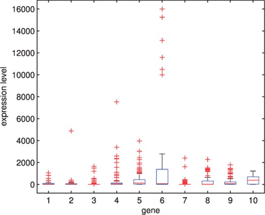
The boxplots for the first 10 genes in the cancer data of Chowdary et al. (2006).

Open in new tabDownload slide

We implemented the MCLUST, MFA, MCFA and MCtFA procedures with g = 2 components with the number of factors q ranging from 1 to 9, using 50 starting values for the parameters. For each value of q, we computed the ARI and the associated error rate. The results are presented in Table 1. We have also listed in this table the values of the BIC and the Approximate Weight of Evidence (AWE: Banfield and Raftery, 1993) for each model with different q. AWE is a model selection criterion based on an approximation to the classification log-likelihood. AWE is defined as

(14)

where EN(τ) = − ∑_j=1ⁿ ∑_i=1^g τ_i(y_j; Ψ)log(τ_i(y_j; Ψ)) is the entropy of the classification matrix with (i, j)-th element equal to τ_i(y_j; Ψ) and m is the number of (free) parameters. It penalizes complex models more severely than BIC, and thus selects more parsimonious models than BIC. It would appear that BIC works well at a practical level; see, for example, Fraley and Raftery (1998). Further, Keribin (2000) proved that BIC provides a consistent estimator of g (Celeux, 2007). But BIC can lead to too few or too many clusters in practice, depending on the problem at hand. For the present problem of choosing the number of factors q, it would appear from Table 1 that it leads to too many factors being fitted in the mixtures of factor analyzers model. An apparent explanation for this is that for the present dataset (and the other one to follow), the data are not well represented by the true models of clusters and/or the true clusters are not well separated. As a consequence, BIC leads to too many factors in the mixture model being fitted to the data. The AWE criterion is preferable to BIC here as it leads to fewer factors since it places a higher penalty on more complex model due to the presence of twice of the entropy and the extra constant term (2EN(τ) + 3m + mlog(n)) in (14). We also considered the ICL criterion which chooses q to minimize −2logL(Ψ) + 2EN(τ) + mlog(n), which is similar to the AWE criterion. They are the same apart from the additional penalty of 3m + mlog(n) imposed by AWE, which for our present problem leads to a better choice of q.

It can be seen that the lowest error rate (0.0288) and highest value (0.8867) of the ARI is obtained by using q = 6 factors with the MCtFA model, which coincides with the choice on the basis of AWE. The lowest error rate (0.1154) of the MFA model is obtained for q = 3 factors. The best result of MCFA model is obtained with its lowest error rate 0.0865 for q = 1 factor (AWE suggests using q = 7). MCLUST chose VVI model as its best and its error rate is 0.3462. It can be seen that the error rate and ARI for MCtFA are better than those for MCLUST, MFA and MCFA. We have also calculated BIC for all models. It can be seen that it failed to select the best model for each method. BIC reached its minimum for largest q (q = 9) of each method, so it selected a more complex model than the one with highest ARI and lowest error rate. In the case where the distribution from which the data arose is not in the collection of considered mixture models, BIC criterion tends to overestimate the correct size regardless of the separation of the clusters (Celeux, 2007).

To illustrate the usefulness of the MCtFA approach for portraying the results of a clustering in low-dimensional space, we have plotted in Figure 2 the estimated factor scores û_j as defined by (13) with the implied cluster labels shown. In this plot, we used the third and sixth factors in the fit of the MCtFA model with q = 6 factors. It can be seen that the clusters are represented in this plot with very little overlap. The estimated factor scores were plotted according to the implied clustering labels. The degrees of freedom of the factor t-distributions for both groups were estimated as 1.0 and 1.0, which means their tails of the distributions are very thick and long. We can easily detect 6 distinct extreme tissues as shown in Figure 2, which are known to be the 9th–14th colon tumor tissue. Figure 3 shows the expression levels of all genes for the 6th–17th colon tumor tissues. In Figure 3, we observe that all of these 6 outliers are very different from others since they have extremely large expression levels not only of the 6th gene shown in Figure 1, but also of other genes.

Fig. 2.

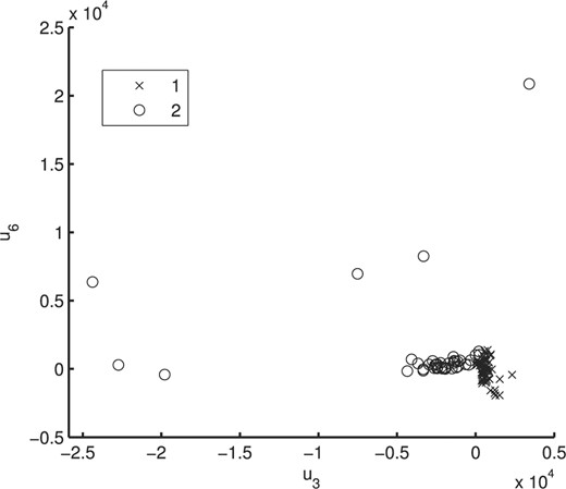
Plot of the (estimated) posterior mean factor scores via the MCtFA approach based on the implied clustering for the cancer data of Chowdary et al. (2006).

Open in new tabDownload slide

Fig. 3.

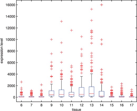
The boxplots of expression levels of all genes for the 6th–17th colon tumor tissues.

Open in new tabDownload slide

The second dataset to which we applied our method is a lung cancer data (Bhattacherjee et al., 2001), for which the number of classes is not small (g = 5). It consists of 203 gene expressions partitioned into five subpopulations: four lung cancer types and normal tissues. Souto et al. (2008) selected 1543 informative genes from the original 12 600 genes. There are big differences among the class sizes of the data. The number of tissues for each class is 139, 17, 6, 21 and 20, respectively. Figure 4 shows the boxplots of the expressions of a gene plotted for each subpopulation. It can be seen that there exist skewed distributions mixed with symmetric distribution with or without extreme observations for five components in the plot. Since the selected (1543) genes are still too many for the mixture model, we grouped the genes into 50 clusters and selected the centroid from each cluster of genes. That is, we applied the k-means algorithm to the 1543 gene expressions and clustered them into 50 groups of similar characteristics. Then we extracted the centroid from each group to make 50 new features for the mixture models.

Fig. 4.

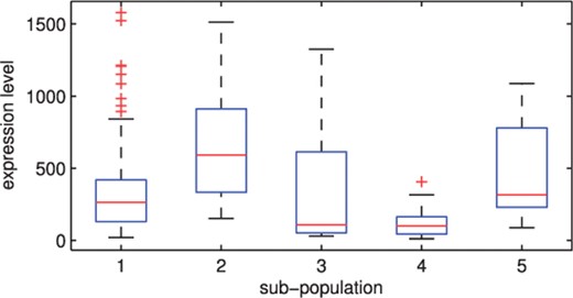
The boxplots for the expressions of a gene by subpopulation: the lung cancer data of Bhattacherjee et al. (2001).

Open in new tabDownload slide

We implemented the MCLUST, MFA, MCFA, and MCtFA approaches with g = 5 components for the number of factors q ranging from 1 to 10, using 50 starting values for the parameters. For each value of q, we computed the ARI and the error rate. The results are presented in Table 2. We have also listed in this table the values of BIC and AWE for each model with different levels of q. MCtFA attains its largest ARI (0.7322) and lowest error rate (0.1133) for q = 6, although AWE suggested the model with q = 7. We notice that there is little difference between the AWE values for q = 6 and for q = 7. The lowest error rate for MCFA is 0.2611 for q = 2 and the largest ARI is 0.4570 for q = 9. The error rate (NA) of MCFA for q = 1 was not able to be calculated since the estimated number of clusters was less than the true value 5. Neither BIC nor AWE indicated the best model for MCFA. MFA reached its best ARI (0.3487) and error rate (0.3498) for q = 7. The minimum BIC and AWE were obtained at q = 6, and at q = 1, respectively. The best model for MCLUST showed similar performance (ARI: 0.3021, error rate: 0.3350) to MFA. MCtFA again performed better than the other methods for this dataset.

We display the data using the estimated factor scores of our model in 3D space (Figure 5). In the latter, we used the second, the fourth and the fifth factors in the fit of the MCtFA model with q = 6 factors. The estimated factor scores were plotted according to the implied clustering labels. It can be seen that the five clusters are represented in this plot with very little overlap. The degrees of freedom of the factor t-distributions for the components were estimated as 1.1, 1.3, 7.8, 4.0 and 4.1. There are two distributions with long tails [ν₁ = 1.1 (triangle), ν₂ = 1.3 (circle)] in the plot. We have also given in Figure 6 the plot corresponding to that in Figure 5 with the true cluster labels shown. There are 23 misallocated tissues which can be seen in other's clusters, but as a whole there is a good agreement between the two plots.

Fig. 5.

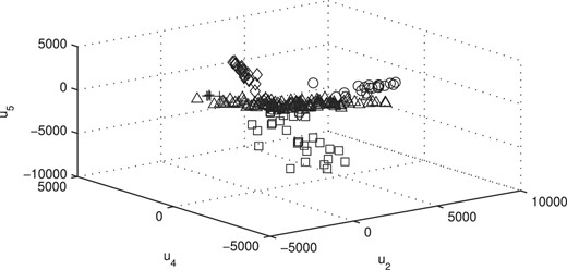
Plot of the (estimated) posterior mean factor scores via the MCtFA approach based on the implied clustering for the lung cancer data of Bhattacherjee et al. (2001).

Open in new tabDownload slide

Fig. 6.

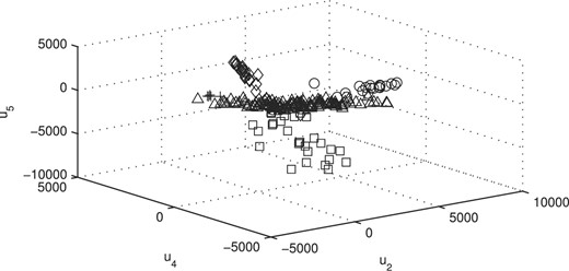
Plot of the (estimated) posterior mean factor scores via the MCtFA approach with the true labels shown for the lung cancer data of Bhattacherjee et al. (2001).

Open in new tabDownload slide

4 DISCUSSION

For clustering high-dimensional data such as microarray gene expressions, MFA is a useful technique since it can reduce the number of parameters through its factor-analytic representation of the component-covariance matrices. However, this approach is sensitive to outliers as it is based on a mixture model in which the multivariate normal family of distributions is assumed for the component factor and error distributions. McLachlan et al. (2007) extended MFA to incorporate t-distributions for the component factor and error in the mixture model for dealing with unusual extreme observations (MtFA). These methods, however, may not provide a sufficient reduction in the number of parameters, particularly when the number of clusters (subpopulations) is not small. In this article, we proposed a new mixture model which can reduce the number of parameters further in such instances and cluster the data containing outliers simultaneously by introducing a mixture of t-distributions with both component-mean and component covariance represented by common factor loadings. We call this approach mixtures of common t-factor analyzers (MCtFA). We describe the implementation of an EM algorithm for fitting the MCtFA. This approach also has the ability to portray the results of a clustering in low-dimensional space. We can plot the estimated posterior means of the factors û_j as defined by (13) with the implied cluster labels. On the other hand, the approaches MCLUST, MFA and MtFA cannot project high-dimensional objects in low-dimensional space. The applications of MCtFA to two cancer microarray datasets have demonstrated the usefulness and its relative superiority in clustering performance over MCLUST, MFA and MCFA. It has shown that our method works well for clustering data containing outliers. Moreover, it provides information on the distribution structure of each subpopulation by displaying the estimated factor scores in low-dimensional space. We observed also that the proposed approach fitted the experimental datasets better than the other approaches, and the performance difference between MCtFA and the others becomes even greater when the number of clusters is not small, such as in the case of second dataset (Section 1.1 of Supplementary Material).

Often BIC is used to provide a guide to the choice of the number of factors q and the number of components g to be used. However, it did not always lead to the correct choice of the best model. That is, BIC can lead to too simple or too complex model in practice, depending on the problem at hand. Simulation studies reported in Biernacki and Govaert (1997), Biernacki et al. (2000) and McLachlan and Peel (2000a) show that BIC will overrate the number of clusters under misspecification of the component density, whereas several alternative criteria such as the AWE and ICL criterion are able to identify the correct number of clusters even when the component densities are misspecified (Frühwirth-Schnatter and Pyne, 2010). In both of our real data applications, we observed that BIC did not choose the best q. An apparent explanation for this is that BIC tries to choose more complex model since some of the subpopulations of the datasets have skewed distributions and have several extreme outliers. On the other hand, AWE leads to the best or almost the best model with smallest error rate since it is more robust against misspecification of the component densities for the experimental datasets. Recently, Frühwirth-Schnatter and Pyne (2010) reported that AWE picked the correct model for both skew-t and skew-normal mixture distributions. Also a small simulation study confirms the better performance of the AWE over the BIC when the distribution of the data has skewed heavy tails due to some extreme observations (Section 1.2 of Supplementary Material). In future work, we wish to investigate the use of various model selection criteria on choosing the number of factors q and the number of components g in mixtures of t or skewed distributions.

Funding: Korea Research Foundation Grant funded by the Korean Government (MOEHRD, Basic Research Promotion Fund, KRF-2007-521-C00048 to J.B.). Australian Research Council (to G.J.M.).

Conflict of Interest: none declared.

REFERENCES

Author notes