


Abstract
Motivation: The careful normalization of array-based comparative genomic hybridization (aCGH) data is of critical importance for the accurate detection of copy number changes. The difference in labelling affinity between the two fluorophores used in aCGH—usually Cy5 and Cy3—can be observed as a bias within the intensity distributions. If left unchecked, this bias is likely to skew data interpretation during downstream analysis and lead to an increased number of false discoveries.
Results: In this study, we have developed aCGH.Spline, a natural cubic spline interpolation method followed by linear interpolation of outlier values, which is able to remove a large portion of the dye bias from large aCGH datasets in a quick and efficient manner.
Conclusions: We have shown that removing this bias and reducing the experimental noise has a strong positive impact on the ability to detect accurately both copy number variation (CNV) and copy number alterations (CNA).
Contact: [email protected]; [email protected]
Supplementary information: Supplementary data are available at Bioinformatics online.
1 INTRODUCTION
Recent advancements in array-based comparative genomic hybridization (aCGH) technology enable entire genomes to be scanned for copy number changes using high-resolution oligonucleotide tiling arrays. In particular, it is now possible to design the content of arrays with a high degree of flexibility as a number of companies offer rapid custom array generation as a standard service. Due to the particular needs of specific experimental questions, microarrays frequently contain oligonucleotide probes displaying variable performance particularly when designs are targeted towards regions of the genome with complex architecture. For example, regions containing repetitive sequences are important for studies of both copy number variation (CNV) and copy number alterations (CNA) and often need to be included in array designs. Replication hot spots contain large numbers of repetitive structures and often underlie the mechanisms for copy number break point formation, which include non-allelic homologous recombination (NAHR), non-homologous end joining (NHEJ), and fork stalling and template switching (FosTes) mechanisms (Gu et al., 2008). Probe performance in and around replication hot spots in repetitive regions is often poor and characterized by heterogeneous probe response. This variable probe response increases the general noise and number of outliers seen across an array, which in turn can cause problems during normalization. With ever-increasing array resolution and complexity, the need for a consistent, efficient, universal normalization method has become of greater importance.
It is well established that a bias exists between the two fluorophores (Cy5 and Cy3) (Chari et al., 2007) due to differential efficiency in enzymatic labelling. This bias manifests as a difference between the two resulting intensity distributions and if left uncorrected is highly likely to skew the ratio calculated during downstream analysis. Over the years there have been a number of different approaches taken for dye bias removal including both linear and non-linear methods (Yang et al., 2002). These methods were primarily developed for the normalization of expression microarrays and have more recently been applied to aCGH microarrays (Staaf et al., 2007). The most commonly used and widely trusted dye bias normalization methods tend to be based on lowess (locally weighted regression) techniques. However, standard regression techniques can be sensitive to outliers, which are common features of aCGH data. As a result, lowess-based dye bias normalization approaches normally use robust regression techniques, becoming computationally intensive and severely limiting if applied to microarrays comprising >300 000 probes (Wang et al., 2004).
Normalization methods based on fitting smoothing spline functions have most often been seen in relation to ‘between-chip’ quantile normalization of microarrays (Skvortsov et al., 2007) and although promising work has been carried out previously (Workman et al., 2002) have thus far seldom been applied to two-colour aCGH microarray data. One possible explanation for this is that when fitting a spline curve only a subset of data is used and without appropriate action can lead to inaccurate data adjustment when applied to complex datasets (Springer et al., 2009).
Here we describe an efficient, robust normalization method using natural cubic spline interpolation (aCGH.Spline), which consistently removes, in a computationally efficient manner, the dye biases seen across a large range of aCGH data.
2 METHODS
2.1 Quality control and outlier exclusion
aCGH.Spline allows the easy processing of data files output from the image analysis software provided by the two major microarray suppliers (Agilent, Santa Clara, CA, USA and NimbleGen, Madison, USA). We support both the reading and writing of the Feature Extraction data format (Agilent), NimbleScan data format (NimbleGen) and a custom data format. aCGH.Spline will automatically flag data points using the image analysis exclusion criteria, which include: spot quality (circularity), spatial effects, low-intensity values and image intensity saturation. To render the method insensitive to outliers and reduce the likelihood of a poor fit and subsequent inaccurate data adjustment, every data point deviating from a defined threshold (see aCGH.Spline Documentation in Supplementary Material) outside of the central distribution of intensity log2 ratios is excluded from the fitting step. The threshold applied to exclude data points within the spline fit is directly linked to the inherent variability (‘noise’) of the dataset. Noise calculation can be performed using two different approaches.
The first approach is to calculate the 68th percentile of the absolute median-normalized log2 ratios between the Cy5 and Cy3 intensities: this value (rp68) is a robust estimation of the experimental log2 ratio variability (Fiegler et al., 2006). The second approach is based on assessing the inter-quartile range between consecutive data points by calculating the derivative log2 ratio spread (dLRs).
Noise estimations of highly complex aCGH datasets (e.g. annioploid samples) can be difficult. Large-scale re-arrangements (CNA's) are likely to produce more then one distinct distribution within a dataset. The ‘rp68’, being based on a Gaussian distribution, is highly likely to report with a falsely elevated value in such cases. As the ‘dLRs’ value is based on the distribution of differences between consecutive data points, it will give a better estimation of the normally distributed noise within such datasets. To further aid in this type of noise estimation, we provide a custom segmentation method to perform an initial change point detection analysis on the raw data values. This allows us to estimate the true baseline or centralized log2 ratio distribution as well as allowing us to assess the log2 ratio distribution as if it were unimodal (see aCGH.Spline Documentation in Supplementary Material).
2.2 Spline fitting
aCGH.Spline is based on a natural cubic spline using Gaussian elimination and backward substitution to obtain the cubic coefficients (Mathews, 1992). The two intensity distributions are fitted independently towards their geometric mean.

The number of knot points and an offset parameter can be adjusted. The offset parameter gives the option of performing a number of spline fits by offsetting the knot points by a given value. If a given set of coordinates (knots points) are {(x0, y0), (x1, y1),…, (xn, yn)}, the required set of n splines are Si(x), i = 0,…, n − 1. These are then computed, using Gaussian elimination, subject to the usual derivative constraints for the splines. Spline interpolation is carried out using the coefficients obtained from each of the offset knot points and the mean result is taken.
2.3 Linear interpolation of outlier values
By using this approach we are able to estimate accurately the adjustment values for all outlier data points without allowing them to affect the overall spline fit.
2.4 Comparison of normalization methods
To assess the quality and speed of our method, we compared aCGH.Spline against four different dye bias removal strategies currently available in R. The four methods are: ‘qspline.normalize’ contained inside the bioconducter package ‘affy’ (Yang et al., 2002), ‘printTipLoess’ contained inside the bioconducter package ‘marray’ (Yang et al., 2002), the ‘popLowess’ method (Staaf et al., 2007) and a simple method utilizing the default ‘Lowess’ function in R. To assess every method reliably, we used 12 replicate experiments run on a custom 244k oligonucleotide whole-genome tiling array, generated by co-hybridizing the well-known samples NA15510 and NA10851 (available at http://ccr.coriell.org).
2.5 Estimation of false discovery rate
To quantify the effect of the different normalization methods on the detection of copy number change point intervals, we estimated false discovery rates (FDRs) by using an ultra high-resolution CGH platform as the gold standard. This platform—the 42M set—consists of a set of 20 NimbleGen arrays containing 2.1 million probes, giving a total of 42 million features evenly spaced across the entire genome with a median coverage of one probe every 56 bp (Conrad et al., 2010). DNA samples from 40 human individuals (including NA15510) were compared to one single reference sample (NA10851) on the 42M set (data provided by the International GSV consortium—http://www.sanger.ac.uk/humgen/cnv/) and CNVs were detected using the genome alteration detection analysis (GADA) algorithm (Pique-Regi et al., 2008).
We then applied six different settings of the GADA algorithm to detect copy number change point intervals from the custom 244k Agilent array. For the six different settings, we constantly kept ‘alpha’ (the sparseness hyperparameter) at a value of 0.1 and varied only ‘T’ (the difference between the sample averages of the probes falling on the left and right segment, divided by a pooled estimation of the standard error) and ‘minL’ (the total number of probes required to detect a change). Settings 1, 2 and 3 had a ‘minL’ of 2 and a ‘T’ of 2, 3 and 4, respectively, whereas settings 4, 5 and 6 had a ‘minL’ of 3 and a ‘T’ of 2, 3 and 4, respectively. As a final step, we also filtered out any change point with an absolute mean ratio of <0.1.
A large number of the features discovered as a result of the 42M study were experimentally validated using either Fluorescence in situ hybridisation (FISH) or PCR (Conrad et al., 2010). The CNV change point intervals from the 42M set were filtered to contain only intervals that could be detected on the 244k Agilent array when applying each of the different GADA settings (Fig. 3A and B). This gave us a minimum functional false discovery resolution of 35.4 kb, equal to one-third of the coverage on our 244k Agilent array (median probe spacing of 11.8 kb). We then compared the intervals detected on the 244k Agilent array against those from the filtered 42M set and calculated both FDR as well as the true and false positive rates as follows:
True positives (TPs) were defined as an interval detected on the Agilent array, which had any overlap with an interval from the filtered 42M set.
False positives (FPs) were defined as an interval detected on the Agilent array that had no overlap with any interval from the filtered 42M set.
True negatives (TNs) were defined as the number of change point intervals seen over the entire filtered 42M dataset (39 samples) that which had no overlap with either the 42M data or the 244k Agilent data for the co-hybridization between NA15510 and NA10851.
False negatives (FNs) were defined as an interval detected on the filtered 42M set that had no overlap with any interval from the 244k Agilent data.
2.6 Comparison with ‘CGHNormaliter’
To highlight the benefits of using aCGH.Spline to remove the dye bias and estimate the true baseline of complex datasets, we compare aCGH.Spline against the recently published ‘CGHNormaliter’ bioconductor package. ‘CGHNormaliter’ was specifically developed to deal with complex datasets and uses an iterative approach (van Houte et al., 2009). We used Case 4 from the ALL lymphoblastic leukaemia dataset (van Houte et al., 2009) to compare the performance of the two algorithms. We ran both CGHNormaliter and aCGH.Spline using their default settings, for aCGH.Spline we then applied the ‘CGHcall’ algorithm (van de Wiel et al., 2007) to the resulting log2 ratio using the same settings as are used by the final change point detection of CGHNormaliter (van Houte et al., 2009). From the resulting ‘aCGHcall’ objects we plotted the data to produce the two Figure 4A and B. We have also produced similar figures for three further cases from the ALL dataset and have included them within the Supplementary Material.
3 RESULTS
3.1 Assessment of normalization quality
We have developed a new normalization method—‘aCGH.Spline’ — to correct dye biases on aCGH profiles. As shown by a number of previous studies, non-linear dye bias normalization methods outperform and add considerable benefit over their linear counterparts (Berger et al., 2004; Wang et al., 2004; Workman et al., 2002; Yang et al., 2002). We have compared aCGH.Spline to four different, freely available, non-linear methods within the R environment. In order to obtain a reliable comparison between the different normalization methods, we used 12 replicate aCGH experiments (NA15510 versus NA10851) on one custom Agilent 244k whole-genome microarray and applied every normalization method to each replicate. Then we compared normalization performances in two different ways.
First, we estimated the inherent variability (‘noise’) of each normalized profile by two independent measurements: the dLRs (the dLRs, a metrics developed by Agilent Technologies) and the rp68 (the 68th percentile of median-normalized absolute log2 ratio values). Secondly, each normalized profile has been analysed using the GADA change point detection algorithm (Pique-Regi et al., 2008), which is available as an R package on the comprehensive R archive network (CRAN). By using an independent set of high-resolution aCGH data as gold standard (see Section 2 for details), we calculated for each profile the CNV FDR, FP rate (FPR) and TP rate (TPR) after applying six different settings of the GADA algorithm (Fig. 3A and B).
For the improvement of inherent experimental variability (‘noise’) across all 12 samples, we see that when using either the robust locally weighted regression methods (‘marray’ and ‘poplowess’) or aCGH.Spline there is a strong decrease in both the dLRs and rp68 value (Fig. 1A and B). When looking at the samples within the middle of the noise distribution (Fig. 1C and D) we see that, for the rp68, there is a strong decrease in noise for all normalization methods with the exception of ‘qspline.normalize’. For the dLRs value we see a less strong, but marked improvement in noise for all normalization methods when compared to using only a global median (Fig. 1B and D).
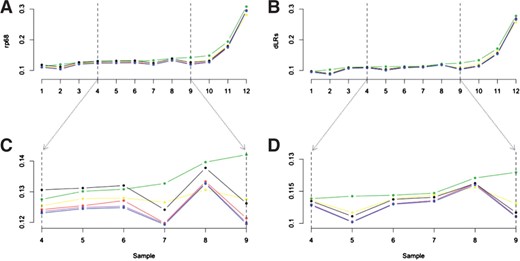
Profile variability over 12 replicate aCGH datasets. Noise values (rp68 and dLRs) over 12 replicate samples when using six different normalization methods are shown. Global median (green), qspline.normalize (black), R Lowess (yellow), popLowess (red), marray (purple) and aCGH.Spline (blue). (A, C) The 68th percentile (rp68) over all 12 replicate samples (A), over six medium-quality samples (C). (B, D) The dLRs over all 12 replicate samples (B), over six medium-quality samples (D).
It is clear that, when using only a global median normalization, dye bias removal will surely be compromised due to not accounting for any non-linear effects (Fig. 2A). Moreover, when using either the global spline fitting method ‘qspline.normalize’ or the locally weighted regression method ‘R lowess’, where no prior outlier exclusion is applied, outlier data points are likely to affect curve fitting, thus resulting, for both methods, in inaccurate adjustment of both outlier and non-outlier data points (Fig. 2B and C). When using the robust regression methods, ‘marray’ and ‘poplowess’, the adjustment of data points are not adversely affected by outlier values; however, the adjustment itself results in the distribution of data points being forced towards a normal distribution (Fig. 2D and E).
![MA-plots [a intensity dependant ratio plot (M is the intensity ratio and A is the average intensity of a dot)] showing normalization quality of Sample 7 when using six different normalization methods. One 244k custom tiling Agilent array under six different normalization methods, autosomes (black), chromosome X (red) and chromosome Y (green) are shown (A) Global median normalization. (B) Standard lowess function in R. (C) ‘qspline.normalize’ method from the ‘affy’ biocondutor package. (D) ‘printTipLoess’ method from the ‘marray’ bioconductor package. (E) ‘popLowess’ method. (F) aCGH.Spline method.](https://oup.silverchair-cdn.com/oup/backfile/Content_public/Journal/bioinformatics/27/9/10.1093_bioinformatics_btr107/3/m_bioinformatics_27_9_1195_f3.jpeg?Expires=1750283362&Signature=N3DB6FbyrhityDqWffbBelHMkTyvagU~xNBYdmsI8zRzoitalgweF~-l8PN59jpEVUqPDN9BbdVmqVQrzWsmsVcqeRMdZ3Cgpd5LO3YwZps5um2ZUBIVNAou1bx1uDIARPzEq1LMH4sqtHRyzKHvzOV7Pz5~gYC6EvlIp9PlUkbirVqJ3~mw9d5yR8VfRTSiv04j5lPqKAzr5QygYRfLVx~X-bn7spSe~JqEYePYoSBqXr9iLZ9g9eo3FArAILr-fQm7725RNJZ3VFKwUHyCw8rgYut5o1MyLJjpYOCcT-XO5eC1EAaZXh7d8n~3AmNiwwXpG0IkFLC4pff0-eC9Zw__&Key-Pair-Id=APKAIE5G5CRDK6RD3PGA)
MA-plots [a intensity dependant ratio plot (M is the intensity ratio and A is the average intensity of a dot)] showing normalization quality of Sample 7 when using six different normalization methods. One 244k custom tiling Agilent array under six different normalization methods, autosomes (black), chromosome X (red) and chromosome Y (green) are shown (A) Global median normalization. (B) Standard lowess function in R. (C) ‘qspline.normalize’ method from the ‘affy’ biocondutor package. (D) ‘printTipLoess’ method from the ‘marray’ bioconductor package. (E) ‘popLowess’ method. (F) aCGH.Spline method.
With aCGH.Spline, by excluding outlier values prior to spline fitting and correcting them by posterior interpolation, we were able to adjust accurately both outlier and non-outlier data points (Fig. 1D). This allows us to retain a distribution of data points closer to the true distribution (Fig. 2A and F) but with most of the dye bias removed (Fig. 2F).
The receiver operating characteristics (ROC) curves based on mean values across the 12 replicates for every GADA setting indicate that aCGH.Spline demonstrates improved sensitivity (TPR) below the 5% FP cut-off when compared to all other normalization methods (Fig. 3B). We also found that on average aCGH.Spline came out top in terms of the reduction of FDRs for each of the GADA settings used (Fig. 3A).
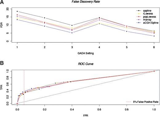
Mean FDR and ROC curve from five different non-linear dye bias normalization methods using six different detection algorithm settings. (A) Mean FDRs after five different normalization methods and six detection settings (GADA) across 12 replicate aCGH profiles. The different GADA settings used are: (i) ‘alpha = 0.1, T = 2, minL = 2’; (ii) -‘alpha = 0.1, T = 3, minL = 2’; (iii) ‘alpha = 0.1, T = 4, minL = 2’; (iv) ‘alpha = 0.1, T = 2, minL = 3’; (v) ‘alpha = 0.1, T = 3, minL = 3’; and (vi) ‘alpha = 0.1, T = 4, minL = 3’. The different normalization methods used are: qspline.normalize (black), R lowess (yellow), popLowess (red), marray (purple) and aCGH.Spline (blue). (B) ROC curves for mean values across the 12 replicate aCGH profiles (HapMap NA15510 versus NA10851) for the five different normalization methods and six GADA settings. TPR (sensitivity); FPR (1-specificity).
Furthermore, aCGH.Spline performed consistently well for the reduction of FDRs for each of the individual samples, the ROC curves and FDR for each individual sample can be found in Supplementary Material (see ROC curves and FDR for 12 replicate aCGH datasets in Supplementary Material). We also observe that overall, across the 12 replicate datasets, aCGH.Spline comes out on top in terms of the reduction of FDR (Table 1) and for Replicate 3 shows a dramatic reduction in FDR compared to all other normalization methods.
FDR following array-CGH data normalization
| Replicate | FDRa | aCGH.Spline | |||
|---|---|---|---|---|---|
| qspline.normalize | rLowess | popLowess | marray | ||
| 1 | 14.035 | 11.321 | 6.000 | 6.000 | 7.843 |
| 2 | 14.286 | 3.509 | 6.452 | 4.918 | 3.390 |
| 3 | 13.158 | 20.000 | 11.111 | 9.091 | 4.878 |
| 4 | 6.667 | 5.085 | 5.000 | 5.085 | 5.172 |
| 5 | 8.772 | 5.000 | 6.154 | 6.250 | 6.250 |
| 6 | 7.143 | 5.660 | 5.357 | 5.263 | 5.455 |
| 7 | 11.475 | 9.434 | 11.667 | 8.621 | 7.143 |
| 8 | 8.163 | 6.522 | 4.545 | 4.545 | 2.273 |
| 9 | 7.937 | 9.091 | 6.849 | 7.042 | 4.615 |
| 10 | 10.000 | 9.211 | 9.412 | 8.974 | 6.579 |
| 11 | 8.955 | 5.634 | 5.479 | 5.556 | 2.941 |
| 12 | 7.143 | 8.000 | 8.750 | 9.333 | 5.714 |
| Mean | 9.811 | 8.205 | 7.231 | 6.723 | 5.188 |
| Median | 8.864 | 7.261 | 6.303 | 6.125 | 5.313 |
aFDR are shown for 12 replicate NA15510 versus NA10851 comparisons on a custom 244k Agilent whole-genome microarray after each normalization method using GADA setting 3 (alpha = 0.1, T = 4, minL = 2).
3.2 Comparison with ‘CGHNormaliter’
Figures 4A and B show that, for Case 4 from the ALL lymphoblastic leukaemia dataset (van Houte et al., 2009), aCGHcall indentifies 14 duplications, most of which were confirmed by FISH, when using data normalized by either CGHNormaliter (van Houte et al., 2009) or aCGH.Spline. However, the probability of each change point (represented by the length of the green bars) is improved when using aCGH.Spline rather than CGHNormaliter. On top of that, normalizing the data using the default parameters for CGHNormaliter results in the incorrect identification of a deletion on chromosome 9. Additionally, both the normalization quality and noise reduction are highly comparable when using either aCGH.Spline or CGHNormaliter.
![aCGHcall detection of Case 4 from ALL (leu) dataset showing the detection probability of 14 experimentally validated duplications using data normalized by either CGHNormaliter or aCGH.Spline. (A) Data normalized by CGHNormaliter using default settings. (B) Data normalized by aCGH.Spline with the ‘segN’ option set to true. Plot resolution is 1:1, the green bars indicating the duplication detection probability and red bars indicating the deletion detection probability. Most of the 14 duplicated chromosomes [4–8, 10–12, 14, 17, 18, 21–23(X)] are confirmed by both CGHNormaliter and aCGH.Spline; however, the aCGH.Spline comes out top in terms of duplication probability.](https://oup.silverchair-cdn.com/oup/backfile/Content_public/Journal/bioinformatics/27/9/10.1093_bioinformatics_btr107/3/m_bioinformatics_27_9_1195_f5.jpeg?Expires=1750283362&Signature=3mqOqlQvrmGSuR2IX5DKFxr-DEVDq-PgWzvUwoAJRtBOet6udCzQwoBkNjTwA8axr2WbiWANZaevE5foRT7qUXK-xIeGxMOfQmscw5OBGk1633W2fkfgGL7XVM5z3qIKMRinNeMGU3ZFSdoZOC3RB6GqQDNE~1tYzeio3j3VzcPkdCPNQ~YIUcm0L8XUL1PHztqGCINhVBNkNKVlikVQAj1zqbwCvgcH0sB7cSbNxZF6oVEEEs~OeEPEswS5hRDXHQ0sbXTNd5qskDTicpAf4KA7FPG5TgAEFOn~xUfdMPembQjTya5HGgsyff8ez0VVJLyCCIBax0Am4UpJDFAULw__&Key-Pair-Id=APKAIE5G5CRDK6RD3PGA)
aCGHcall detection of Case 4 from ALL (leu) dataset showing the detection probability of 14 experimentally validated duplications using data normalized by either CGHNormaliter or aCGH.Spline. (A) Data normalized by CGHNormaliter using default settings. (B) Data normalized by aCGH.Spline with the ‘segN’ option set to true. Plot resolution is 1:1, the green bars indicating the duplication detection probability and red bars indicating the deletion detection probability. Most of the 14 duplicated chromosomes [4–8, 10–12, 14, 17, 18, 21–23(X)] are confirmed by both CGHNormaliter and aCGH.Spline; however, the aCGH.Spline comes out top in terms of duplication probability.
As a result of the iterative nature of the CGHNormaliter method (van Houte et al., 2009), it has become computationally demanding and even when applied to a relatively small number of data points (<32 000) is considerably slower than aCGH.Spline.
3.3 Computation speed
We measured the time required by aCGH.Spline to process a variety of array formats as well as the number of outlier interpolations performed (Table 2). In R 2.10, running on a MacBook4.1 Intel Core 2 Duo (2.1 GHz), aCGH.Spline takes on average 69 s (including file reading and writing) to process an Agilent Feature Extraction file containing 244 000 data points (performing 4820 outlier interpolations) and 499 s to process an Agilent Feature Extraction file containing 1 million data points (performing 30 404 outlier interpolations).
Computational speed of aCGH.Spline
| Replicate | 44ka | 105k | 180k | 244k | 1M | |||||
|---|---|---|---|---|---|---|---|---|---|---|
| Interb | sc | Inter | s | Inter | s | Inter | s | Inter | s | |
| 1 | 752 | 10 | 476 | 29 | 72 | 32 | 94 | 42 | 3907 | 289 |
| 2 | 95 | 14 | 710 | 33 | 111 | 32 | 136 | 46 | 4821 | 301 |
| 3 | 924 | 16 | 1066 | 35 | 552 | 33 | 962 | 58 | 4807 | 311 |
| 4 | 792 | 17 | 479 | 36 | 175 | 37 | 677 | 62 | 12 242 | 335 |
| 5 | 162 | 17 | 608 | 36 | 2460 | 39 | 1147 | 65 | 11 032 | 395 |
| 6 | 321 | 17 | 653 | 37 | 2571 | 39 | 2166 | 65 | 13 632 | 457 |
| 7 | 659 | 18 | 946 | 37 | 2660 | 39 | 2504 | 71 | 58 693 | 699 |
| 8 | 1014 | 18 | 2415 | 39 | 2271 | 43 | 12 986 | 85 | 61 200 | 709 |
| 9 | 1716 | 18 | 1069 | 39 | 8706 | 51 | 9423 | 90 | 57 784 | 711 |
| 10 | 1098 | 20 | 2418 | 40 | 9671 | 58 | 13 814 | 92 | 61 823 | 721 |
| 11 | 808 | 17 | 489 | 37 | 178 | 38 | 691 | 63 | 12 487 | 342 |
| 12 | 1034 | 18 | 2463 | 40 | 2316 | 44 | 13 246 | 87 | 62 424 | 723 |
| Mean | 781 | 17 | 1149 | 36 | 2645 | 40 | 4820 | 69 | 30 404 | 499 |
aMicroarray size, in number of oligonucleotide probes.
bNumber of outlier interpolations in aCGH.Spline to fully process a Feature Extraction file.
cTotal processing time in seconds.
To assess the speed performance of aCGH.Spline against the other non-linear normalization methods, we computed the mean time taken by each method to process the 12 replicate 244k custom Agilent arrays. The ‘R lowess’ method took an average of 42 s and the ‘qspline.normalize’ method took an average of 46 s to process 244 000 data points; this level of performance was expected as neither method is fully robust to outliers. The two robust regression methods did not fair so well, the ‘printTipLoess’ method from ‘marray’ taking on average 482 and the ‘popLowess’ method 318 s to process 244 000 data points. We also calculated the time taken by ‘CGHNormliter’ to process the 244k Agilent arrays, taking on average 1923 s (32 min).
4 DISCUSSION
In this study, we have shown that aCGH.spline enables efficient dye bias removal on aCGH profiles, giving similar, if not superior, results to several approaches available within the R programming environment (Staaf et al., 2007; van Houte et al., 2009; Yang et al., 2002). Interestingly, aCGH.Spline not only increases data quality by reducing the experimental noise (Fig. 1), but also decreases the FDR (Fig. 3 and Table 1) in the majority of situations. Removing a large portion of the dye bias reduces the inherent noise of aCGH profiles and decreases the magnitude of falsely elevated or lowered log2 ratio values (Fig. 2).
Estimating experimental variability can be difficult with highly rearranged or aneuploid samples where the majority of data points respond to an altered copy number state, thus falsely increasing noise estimations (Neuvial et al., 2006; Oshlack et al., 2007; Springer et al., 2009; Staaf et al., 2007; Yang et al., 2002). We chose to use two different estimations of the systematic noise in aCGH profiles: (i) the rp68 (68th percentile of the absolute log2 ratio values), which gives an accurate estimation of the spread of the noise within the centralized log2 ratio distribution; (ii) the dLRs that measure the probe-to-probe noise across the array. Although both of these measures are, to some degree, insensitive to outliers, using a combination of the two is necessary for accurate quality control of aCGH data. Indeed, by using the dLRs value alone as a quality control (QC) metric, it is possible to miss subtle artefacts within the dataset. For example, the auto-correlation or ‘wave’ profile often seen in aCGH data (Marioni et al., 2007) will not be well reflected by a dLRs value. Additionally, by using only the rp68 value as a QC measure, the noise estimation of highly variable datasets (e.g. annioploid samples) can be compromised.
As the use of ultra-high-resolution microarrays becomes a standard for aCGH analysis, it is important to be aware of the potential for increased FDRs. Using a custom microarray comprising 1 million probes in our hands leads to the detection of >1000 CNVs. With a FDR of 5% (which is usually considered as an acceptable cut-off) this analysis would include 50 false discoveries. Decreasing FDRs is of great importance for the identification of CNVs associated with disease or evolution and for avoiding unnecessary and wasteful validation of results.
aCGH.Spline is efficient for the normalization of arrays with >1 million data points and performs consistently over a range of data complexities (Figs 1, 2, 3 and 4). This method is particularly useful for the processing of large numbers of ultra-high-resolution microarray datasets (Table 2). Although all of the results presented here have been generated using Agilent aCGH arrays, the method can be applied to any dual colour microarray data. The aCGH.Spline R package contains various functions for the reading and writing of standard microarray data formats, including the complex feature extraction data format from Agilent, the generation of QC statistics and the plotting of data. The package is deliberately distributed with mild default parameters (see aCGH.Spline Documentation in Supplementary Material) and aims to include only data points that are representative of the dye bias within the spline fit. This reduces the likelihood of inaccurate adjustment of the data and tends to decrease the FDR (see Fig. 3 and Table 1).
We are currently developing other methods to further improve the quality of aCGH data and remove some commonly observed artefacts; these new methods require some prior knowledge about array design and performance. The aCGH.Spline normalization method can be used to remove the dye bias from any aCGH profile and thus improve data quality without the need for any prior understanding of array performance characteristic.
Effective normalization of aCGH data is of great importance for inferring accurate estimations of copy number change (Oshlack et al., 2007; Staaf et al., 2007; Workman et al., 2002; Yang et al., 2002). Here, we demonstrate that the aCGH.Spline method removes most of the dye bias seen between the two fluorophores Cy5 and Cy3 and results in a decrease in both the experimental noise and copy number change point FDR. Compared to Lowess-based methods (Staaf et al., 2007; van Houte et al., 2009; Yang et al., 2002), the most widely used of normalization strategies for the reduction of the dye bias seen within aCGH data, aCGH.Spline demonstrates improved normalization performance as well as a reduction in computation time.
The aCGH.Spline method has been written in R and Java and submitted to the R-project as a package, available at http://cran.r-project.org. The distributed version of the R package utilizes the ‘rJava’ package and draws upon methods contained inside a Java class to increase speed performance. A Java GUI will be available soon, which allows the processing of most standard array data formats within an easy to use interface.
ACKNOWLEDGEMENTS
We would like to thank the International GSV consortium for the availability of high-resolution CNV data (http://www.sanger.ac.uk/humgen/cnv).
Funding: This work was supported by the Wellcome Trust (grant number WT077008).
Conflict of Interest: none declared.
REFERENCES
Author notes
Associate Editor: Martin Bishop

