Automated analysis of biological oscillator models using mode decomposition Free

Abstract

1 INTRODUCTION

Oscillations are observed in biological systems at various levels ranging from molecular through cellular to population (Goldbeter, 2002; Novak and Tyson, 2008). Such signals offer a means to collect non-redundant data from single systems and thereby present opportunities for studying generating mechanisms. Indeed, it has recently been argued that analysis of oscillatory gene expression profile shapes can distinguish between, i.e. validate or invalidate, candidate theoretical models (Konopka and Rooman, 2010). It is not unreasonable, therefore, to hope for gaining sufficient understanding of the processes involved to predict their behavior under novel circumstances, which may be useful for example for synthetic biology. These observations provide motivation for developing techniques and software tools to facilitate and to automate the analysis of such signals.

A well-known technique for analyzing oscillating signals is Fourier analysis [e.g. (Gray and Goodman, 1995)]. Two of its main results state that an oscillating signal with base frequency ω can be expressed as a sum of sine and cosine modes with frequencies ω, 2ω, 3ω, etc. and that the amplitudes of each of these components can be computed from the signal's time-series using an efficient algorithm. In practice, only a small number of these amplitudes need be known to describe a typical signal, and they can be estimated with good accuracy if the signal time-series has a large number of points. These properties have previously been applied in several engineering applications, [e.g. (Gray and Goodman, 1995; Lembregts et al., 1990)]. In the context of bioinformatics, Fourier-based techniques have been used for the identification of genes showing oscillatory behavior in microarray data (Shedden and Cooper, 2002; Spellman et al., 1998; Whitfield et al., 2002; Wichert et al., 2004 and for their subsequent clustering/analysis (Feng et al., 2009; Kim and Kim, 2008).

Many theoretical models proposed in the literature to describe biological oscillators contain non-linear equations (Goldbeter, 2002; Novak and Tyson, 2008). Such equations produce signals with distinctive patterns of harmonic components in their Fourier spectra. Detection of these patterns in experimental data can, therefore, be used to distinguish between different candidate models. On this basis, a particular pattern of mode amplitudes in a dataset on circadian oscillations (Hughes et al., 2009) was recently argued to be inconsistent with two model structures (Konopka and Rooman, 2010). The invalidation was performed despite that both models were able to produce periodic waveforms of the observed base frequency.

The aim of this work is to generalize and systematize the model validation and invalidation approach based on the frequency domain. That is, the goal is to develop a method for suggesting mathematical descriptions for time-series given a set of observed signals. The method should not only determine whether a proposed model structure is consistent with observations, but also scan a number of alternative models.

In general, the problem of ab initio identification of mathematical descriptions for time-series is a very difficult one (Džeroski and Todorovski, 2008; Gennemark and Wedelin, 2009). Two main reasons for this are as follows: (i) there is a need to specify the type of equations structures to be studied and (ii) it is necessary to determine which of the equations are good descriptions for data. The first issue is non-trivial since there are a priori an infinite number of possible model structures that might be considered. It is addressed here by defining finite classes of equations relevant for biological oscillators. The second issue can be a hindrance for model identification because it usually involves fitting values of unknown parameters, which can be computationally expensive and can moreover lead to ambiguous outcomes if models are underdetermined (Ljung, 2010; Zheng and Sriram, 2010). In this work, this difficulty is avoided by restricting attention to oscillatory signals and exploiting the structure of the relevant equations as well as the properties of the frequency-domain signal decomposition.

The class of model structures considered in this work is a subset of first-order ordinary differential equations, which involve a primary signal φ(t) driven by another signal ψ(t). The types of interactions and the number of free parameters entering in the equations is restricted, but are defined as to include biologically/chemically relevant interactions such as Hill or Michaelis–Menten kinetics. When interpreted in the context of gene expression models, the equations can describe promotion/inhibition effects by activating factors, removal by polymerase or membrane channels, degradation, monomeric/dimeric effects, etc. They can be used to study entire systems proposed in the literature, including the Lotka–Volterra oscillator of ecology, the Goodwin (Goodwin, 1965) or the Novak–Tyson oscillators (Novak and Tyson, 2008) describing RNA and protein levels in cells.

In what follows, Section 2 defines the class of equations considered in this work in more detail and describes the workflow for model selection. The workflow is applied to datasets in Section 3: some generated synthetically and one from the literature on circadian oscillations (Hughes et al., 2009). Section 4 summarizes the results and offers some perspectives.

2 METHODS

2.1 Enumeration of model structures

The class of model structures considered in this work is that of ordinary differential equations involving a primary signal φ(t) and a driving signal ψ(t) and that can be written as

(1)

where t denotes time and ⁠. The functions W_1,2 on the right-hand side are required to be chosen from the set in Table 1 with the further condition that ψ(t) appear at least once in the equation. Intuitively, the role of one of the W terms is to make the signal grow during the first part of an oscillation cycle while the role of the other is to later drive the signal back down.

Table 1.

Open in new tab

Taxonomy of terms to appear in model equations

Term .	Expression .	Term .	Expression .	Term .	Expression .
1	k  1	5		9
2	k  1φr	6		10
3	k  1ψs	7		11
4	k  1φrψs	8		12

Term .	Expression .	Term .	Expression .	Term .	Expression .
1	k  1	5		9
2	k  1φr	6		10
3	k  1ψs	7		11
4	k  1φrψs	8		12

k  ₁ and k₂ are free parameters. Integers r, s set the orders of interactions for signals φ and ψ, respectively.

Table 1.

Open in new tab

Taxonomy of terms to appear in model equations

Term .	Expression .	Term .	Expression .	Term .	Expression .
1	k  1	5		9
2	k  1φr	6		10
3	k  1ψs	7		11
4	k  1φrψs	8		12

Term .	Expression .	Term .	Expression .	Term .	Expression .
1	k  1	5		9
2	k  1φr	6		10
3	k  1ψs	7		11
4	k  1φrψs	8		12

k  ₁ and k₂ are free parameters. Integers r, s set the orders of interactions for signals φ and ψ, respectively.

The terms in the table are all the possible ones that satisfy the criteria: they are fractions wherein both the numerator and denominator are polynomials in the signals, they contain at most two free parameters each, the denominator depends on only one of the signals and the power (order) of each signal appears consistently in the numerator and denominator. When the maximal orders r, s for each term are set to 1 or 2, the number of distinct equations in the classes are 60 or 507, respectively. The number of free parameters in each equation is at most equal to four.

Each member Equation (1) can be interpreted as a biological process. For example, taking W₁ and W₂ of types 2 and 3 with orders set to 1 (Table 1) leads to the equation ⁠, where p₁ and q₁ are parameters taking the place of k₁ in the table. When p₁ < 0 and q₁ > 0, this might be used to describe RNA concentration of gene φ, which decays at a rate proportional to φ and is replenished at a rate proportional to the concentration of a promoting factor ψ. Replacing the term of type 3 in this example by a term of type 11 would introduce a saturation or rate-limiting effect to the replenishing mechanism familiar from Michaelis–Menten kinetics.

The remainder of Section 2 deals with fitting time-series for signals φ(t) and ψ(t) to equations of type (1). The discussion demonstrates how the unknown parameters in each equation of the class can be estimated efficiently, and how the results can reveal the suitability of each equation to describe the data. The methodology thus consists of an exhaustive search over the class of equations and outputs the subset that is consistent with the data.

2.2 Parameter estimation using mode decomposition

Because all the terms in Table 1 can be written as fractions wherein both the numerator and the denominator are polynomial in the signals, it is convenient to rewrite Equation (1) as

(2)

Here, p_1,2 and q_1,2 are independent parameters replacing k_1,2 in the table, and r_1,2 and s_1,2 are integers replacing r and s. Multiplying out the denominators, suppressing the dependencies of f₁₋₄ and rearranging yields

(3)

This step resembles a systems identification procedure called complexification (Ljung, 2010; Ljung and Glad, 1994).

A signal φ(t) that oscillates with base frequency ω can be described using mode decomposition as

(4)

where μ_n ∈ R and ν_n ∈ R are coefficients that can be computed from a time-series using the Fourier transform (Supplementary Material). A signal ψ(t), which is required to oscillate at the same base frequency, can be expanded in an analogous way with a different set of coefficients. In practice, only a finite number of coefficients might be available so decompositions such as (4) would be truncated to a finite length. The remainder of the analysis assumes that such truncated series are good approximations to the real signals.

Expansions for φ(t) and ψ(t) can be substituted into a model Equation (3) as trial solutions. Because of the form of the signal expansion (4) and the polynomial nature of the model equation, the sole dependence on t in the result is through factors such as e^inωt. A replacement e^iωt → z turns it into an algebraic equation in z,

(5)

Equating coefficients of z on the left and right-hand sides gives Reλ_n=0 and Imλ_n=0 for all n, which imply relations among the parameters p_1,2, q_1,2. In principle, there is an infinite number of such relations. In practice, the number is limited by the truncation levels of the mode decompositions. All relations are polynomial in the parameters and hence readily solvable either analytically or numerically.

Three distinct situations may arise during the parameter identification step. If the number of unknown parameters is greater than the number of relations extracted from (5), there is no unique solution. If the two numbers are equal, one or multiple sets of parameter values may be computed depending on the type of model equation being considered.

The third situation occurs when the number of relations is greater than the number of parameters. Parameters may then be solved for several times using independent relations. For example, for a model with two unknown parameters, relations Reλ₁=0 and Imλ₁=0 arising from the z¹ coefficient can be used to compute one set of parameters. Then, relations Reλ₂=0 and Imλ₂=0 from the z² coefficient can be used to compute another set of parameters, and so on. The choice of coefficients and relations can be termed as the depth or level at which the parameter estimation procedure is carried out.

2.3 Selection of solutions

Numerical estimates for the parameters can subsequently be used to determine whether a particular model is a good description of the observed signals. On physical grounds, all parameters should have real values. However, since they are obtained by solving polynomial equations, they are generally found to have imaginary components. This can be attributed to noise in measurement of the original signals, approximation of the signals via decomposition (4) or numeric issues while solving the coefficient equations. It can also be an indication of inconsistency of the trial solutions with the model equation. Thus, while small imaginary components might be ignorable, a given parameter set should be rejected if the imaginary components are too great compared with the real ones. This can be dealt with via tolerance levels. For example, with a tolerance to imaginary components of X, a parameter value p₁ can be accepted if |Imp₁| < X|Rep₁| and rejected otherwise. Rejection of one parameter implies rejection of the entire model equation. All further discussion always refers to the real components of parameter values.

Another very fast method to eliminate candidate model structures is to specify physically acceptable ranges for the parameters and check whether the computed solutions lie within these ranges. Part of this step is subjective and depends on the scale or units used in the time-series. However, some selection is possible on theoretical grounds. In particular, the parameters that appear in the denominators in Table 1 are always positive definite in physical models and indeed must be so in order for the proposed methodology to be well defined. Solutions violating this condition can be rejected.

When several parameter sets can be computed redundantly from coefficients of different powers of z, they must include a self-consistent set if the signals and model structures are compatible. In practice, the redundant solutions are never identical because of the sources of error mentioned above and consistency must again be defined according to some tolerance levels. Since estimates for parameter values obtained by equating coefficients of low-order coefficients (z⁰, z¹) are generally most reliable, these parameters are defined as the reference set. Parameter sets obtained from higher order coefficients (z², z³, etc.) can then be compared with the reference set. If the latter match the reference set within some tolerance levels, the model structure can be accepted. For example, a parameter p₁ appearing in a model equation might be evaluated to a value p₁⁽¹⁾ using low−order coefficients (depth level 1) and to a value p₁⁽²⁾ using higher order coefficients (depth level 2). Here p₁⁽¹⁾ is the reference value. With a tolerance level of Y, the two estimates would be considered consistent if (1 − Y)p₁⁽¹⁾ < p₁⁽²⁾ < (1 + Y)p₁⁽¹⁾ (inequalities are reversed if p₁⁽¹⁾ < 0).

In many cases, these selection criteria are sufficient to reduce the number of candidate model structures from several hundreds to single digits. The remaining solutions may be further checked by reconstructing a signal φ using the driving signal ψ, an initial condition for φ, the model equation and its estimated parameter set. A correct model structure should produce a signal that closely matches the original as quantified via an objective function such as the average squared error. This criterion is effective in selecting among a small number of model structures but is more computationally expensive to implement than the previous criteria.

All procedures, parameter estimation as well as model selection, can be automated for the class of equations defined in Section 2.1. An implementation for Mathematica is made available through a package described in detail in the package documentation.

3 RESULTS

3.1 Model reconstruction from ODE simulations

To demonstrate the parameter estimation and model selection procedure and to illustrate its strengths and limitations, it is applied to a set of signals generated in silico. The system studied is defined by eight signals ϕ₁₋₈ satisfying:

(6a)

(6b)

(6c)

(6d)

(6e)

(6f)

(6g)

(6h)

The first four signals, ϕ₁₋₄, reproduce a model defined in (Novak and Tyson, 2008) describing concentrations of RNA and protein in two cellular compartments. They produce sustained oscillation patterns via a closed loop of promoting and inhibiting actions. Signal ϕ₅ oscillates because it is driven by ϕ₄ from the previous group. Signal ϕ₆ is defined in terms of a random variable ξ(t) drawn from a normal distribution. It is a random walk and is thus not oscillatory; it acts as a decoy. Finally, ϕ₇ and ϕ₈ correspond to the Lotka–Volterra oscillator used to model predator–prey dynamics in ecology. These signals produce oscillations independently from ϕ₁₋₅. Together, Equations (6a)–(6h) involve a varied selection of terms from Table 1.

The numerical values for parameters k₁₋₁₀ and the initial conditions for ϕ₁₋₄ are set in ranges close to those in Novak and Tyson (2008). The remaining parameters and initial conditions are chosen by hand. For the Lotka–Volterra oscillator, g₁₋₄ are set as to make ϕ_7,8 oscillate with the same fundamental frequency as ϕ₁₋₅. The system is solved numerically with fine temporal resolution until steady oscillations are reached. A portion of this signal is then subsampled to yield a series with 108 points and six complete cycles per signal. The short signals are then passed though a noisy channel of varying strength. Below, two such datasets are used: the first set is noiseless and the other has 6% normal noise. Other noise levels (levels tested up to 10%), whether introduced in the time-series or spectral representations, produce qualitatively similar results (data not shown). Different instantiations of noise also yield qualitatively similar results (data not shown). Further details on simulations and results are given in the Supplementary Material.

All signals' Fourier spectra are computed using standard methods and they are then considered pairwise. For each pair, all the equation structures defined in Section 2.1 with maximal orders r, s = 2 are tested (507 equations per signal pair, or 32 448 in total). The depth level for parameter estimation is capped at 2. Thus, two sets of parameters are computed for each model structure. Tolerance across the depth levels is set to 50%, and tolerance levels to imaginary values are set to 50% and 100% at depth levels 1 and 2, respectively. Comparison of parameter sets with these tolerance levels is then used to accept or reject candidate model structures.

A summary of the results is shown in Figure 1. In both Figure 1A and B, the rows and columns represent driving signals ψ(t) and primary signals φ(t), respectively. Numbers in the cells show how many model structures pass the selection criteria. For example, the items in the third column and second row represent results of calculations testing model structures with φ(t) = ϕ_3(t) and ψ(t) = ϕ_2(t), i.e. equations of type (1) with on the left-hand side. The numbers 4 and 2 indicate that many equations are consistent. At the same time, the numbers mean that 503 (= 507−4) and 505 (= 507−2) other equations are rejected.

Fig. 1.

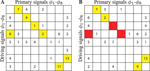
Model reconstruction from synthetic data. The tables list the number of model structures consistent with the synthetic data, signals ϕ₁ to ϕ₈. Rows denote driving signals, ordered from top to bottom. Columns denote primary signals, ordered from left to right. Yellow (Red) cells indicate that one (none) of the accepted equation structures corresponds to the one actually used to generate the signals. (A) Results using noiseless signals. (B) Results using signals with 6% normal noise.

Open in new tabDownload slide

When the input data is of excellent quality (Fig. 1A), the model selection criteria can be made strict enough to eliminate all but a handful of incorrect models. The remaining model structures are consistent with Equation (6). When the data are noisy (Fig. 1B), the results are poorer but still informative. The figure shows some red cells, which indicate that correct model structures are rejected according to the chosen criteria. Given estimates of distinct peaks in the signals' spectra (see Supplementary Material), this should not be too surprising; attempting to estimate model parameters using amplitudes that are too noisy can confuse the selection criteria. This shows that choosing appropriate depth levels and selection criteria are important steps in the analysis.

Figure 2 shows some comparisons between the noisy signal curves and their reconstructions computed using equations and parameters sets outputed by the automated procedure. As a reference, Figure 2A represents one of the cases where the correct model structure and associated parameters are used to compute the smooth curve. The match between the original and reconstructed signals is understandably quite good. In Figures 2B and 2C, the curves describe primary and driving signals that are related in Equation (6), but where the equations used in the reconstruction are different from Equation (6). The actual and reconstructed curves match well in the first but not in the second. The latter model can thus be rejected on grounds of the time-domain plot. Finally, Figure 2D shows a proposed relationship between a set of signals that are not directly coupled in system (6). However, the match between the curves is not unacceptable in an obvious way.

Fig. 2.

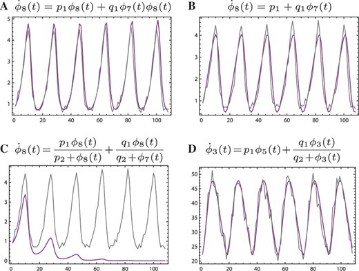
Signals reconstructed from computed parameter sets. Jagged gray lines are the noisy synthetic data. Smooth purple lines are signals reconstructed using equation structures and parameter values suggested by the automated model selection method. All panels show signal intensity versus time (all units arbitrary).

Open in new tabDownload slide

Figure 2B exemplifies that an observed signal pair can sometimes be described by more than one equation structure. Figure 2D shows that a physically non-existent interaction can be modeled by a fairly simple equation. Both are, therefore, reminders that fitting a single particular proposed model to a set of measurements cannot be sufficient to claim an understanding of a biological process. It is reassuring, however, that many such ambiguities can be resolved by improving the resolution and quality of the input data. The model in Figure 2B is, in fact, rejected when using less noisy data and more stringent selection criteria (data not shown). The model in Figure 2D, however, persists so different techniques may be needed to invalidate it. In an experimental context, these may involve collecting new data under different environmental conditions or exploiting a mutant system (Konopka and Rooman, 2010).

The time-domain selection criterion can be automated just like the parameter computation procedure. This involves integrating each of the equations that pass the previous round of selection criteria and then computing the mean error between the original and reconstructed signals. Thresholds of 2% and 6% of the wave maximum to minimum intensity difference are set as for the noiseless and noisy signals sets, respectively.

Results after time-domain selection are shown in Figure 3. In comparison to Figure 1, numbers in many of the cells are reduced or set to zero. This exemplifies that the time-domain technique can usefully complement the selection criteria applied previously. This is useful, but the computation overhead to produce the time-domain reconstruction and to calculate the mean error can be considerable compared to the other model selection steps.¹ For this reason, the time–domain error technique is best applied at the last stage of analysis when only a small number of model structures need be considered.

Fig. 3.

Model reconstruction from synthetic data after frequency-domain and time-domain selection. (A) and (B) are analogs of Figures 1A and 1B after time-domain selection.

Open in new tabDownload slide

To conclude this section, the issue of rejection of correct model structures (red cells) is revisited. To avoid such erroneous results, the workflow can be run multiple times on datasets artificially corrupted by additional noise. Adding more noise produces signals whose spectra are sometimes closer to the true ones and hence allow the acceptance of the correct model structure. This technique is discussed further in the Supplementary Material.

3.2 Model reconstruction from stochastic simulations

Because the number of molecules participating in chemical reactions in cells is usually small, cellular processes are subject to intrinsic stochastic noise [see e.g. (Paulsson, 2005) for a review]. Signals produced by these processes may thus be more accurately described by synthetic signals produced via stochastic simulations using the master (Paulsson, 2005) or the Langevin equation approaches (Gillespie, 2000) rather than ordinary differential equations with noise added in post-processing. To investigate these issues, a similar analysis as above can be repeated for signals generated by stochastic methods. The results are presented in the Supplementary Material. Briefly, they show that the methodology works similarly as above but is subject to an important caveat.

Oscillatory signals produced in strongly stochastic simulations are more irregular than those obtained from ODEs. The amplitudes of their cycles and the time interval between maxima can be variable (Gonze et al., 2002). As a result, their spectra can have broad rather than sharp peaks. This implies the expansion (4) with a small number of terms becomes a less appropriate description of the signals. For long time-series, the effect is significant and has a detrimental effect on the parameter estimation and model selection procedure. For short time-series, however, for example those covering only two cycles, the items of the spectrum used in the parameter estimation procedure capture sufficient information about the signals to make reconstruction feasible.

3.3 Model identification for circadian oscillators

The automated model selection analysis can be applied to experimental data. An interesting data set on oscillators is from a micro-array experiment on the circadian cycle in mouse liver cells (Hughes et al., 2009). It includes measurements of expression levels for over 40 000 probesets (genes) collected at 1-h intervals over the course of 2 full days. About 4000 of these signals contain oscillatory components. The same dataset was used previously to point out that some gene expression patterns show interesting patterns in their Fourier spectra that can be used for model selection (Konopka and Rooman, 2010).

An important complication for model selection that arises with micro-array data is signal filtering (Supplementary material). Intensity levels measured in microarray probeset are functions of the probe–target binding propensity as well as of the real RNA concentration. Indeed, this effect can be detected by comparing profiles of the same gene as measured in different probesets (Supplementary Material). In what follows, however, the effect is not explicitly dealt with for two reasons. First, proper accounting of filtering is difficult as the effect is not the same for all probesets. Second, some simple filters should not affect the ability of the methodology to detect consistent equations. Model selection calculations may, therefore, still be useful with the filtered signals, although the results should be interpreted with the effect in mind. In particular, numerical values of estimated parameters should not be overemphasized.

Since the number of probesets with oscillating profiles is on the order of thousands (Hughes et al., 2009), a brute-force approach considering all possible models and all possible probeset pairs is not feasible even with the fast frequency-domain method. The approach taken here is, therefore, to select a small subset of genes on the basis of number of peaks in the spectra that are a certain amount above the noise level (see Supplementary Material). Such signals are least prone to give erroneous results. Because of noise and the still large number of signal pairs, testing is restricted to models with maximal interaction order equal to one. Model selection is repeated five times with additional noise added in each round to reduce the impact of the problems discussed at the end of Section 3.1. Selection criteria are set similarly as in the previous sections.

Detailed results appear in the Supplementary Material. In brief, 33 signals coding for 30 genes are retained after selecting for number of spectral features. The model selection procedure suggests 452 model structures relating several signal pairs (the number of considered models is 65 340, each evaluated five times using slightly different data). Most often, the structures involve terms of type 1−4 from Table 1, i.e. terms that are non-fractional. This suggests that saturation effects might not be important in the dynamics of the considered genes, or that such effects are not well captured by equations with reaction orders equal to one. Among the terms of type 1−4, signal decay is suggested to take place by several mechanisms: proportional decay, constant removal, as well as following a predator–prey relationship with driving signals.

Another general observation is that some signals have much higher propensity to be selected as driving signals than others. The two most active signals in this sense are Slc25a32 and Pim3, coding for a mitochondrial folate carrier and for a protein kinase, respectively. In some cases, more than one gene is suggested to affect a certain signal. For example, Figure 4 shows examples where the two mentioned genes drive signal Timm8a1, coding for a mitochondrial membrane protein. In both cases, the equation is

(7)

and the parameters satisfy p₁ < 0 and q₁ > 0. This suggests that the driving signals are promotors of Timm8a1, decay is of exponential type and there are no significant saturation effects taking place. In reality, both models are unlikely to be true simultaneously, and it would be necessary to use expert knowledge on gene function or further experimentation to eliminate one (or both) of them.

Fig. 4.

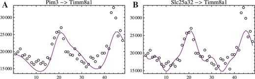
Examples of reconstruction of circadian oscillation signals. Both panels show reconstructions of the expression profile of gene Timm8a1 (intensity in arbitrary units versus time in hours) driven by (A) gene Pim3 and (B) gene Slc25a32.

Open in new tabDownload slide

The curves in Figures 2 (also in Fig. 4) are computed using parameters outputted from the lowest depth level and the earliest time-point of a time-series as an initial condition. They satisfy all the criteria set at the start of the calculation, but they are not fitted in the sense of having had been adjusted to minimize an objective function. The fits, therefore, could be improved by tuning the parameters using conventional (Ljung, 2010; Zheng and Sriram, 2010) or approximate (Cao and Zhao, 2008) methods at the cost of additional overhead.

4 CONCLUSIONS

To summarize, this work defines an automated workflow for the analysis of oscillating signals originating from biological or chemical systems. The methodology deals with questions of recognized interest in systems biology: determining mechanisms and associated equations that might be responsible for observed phenomena [e.g. (Gennemark and Wedelin, 2009; Marbach et al., 2010)]. Attention is restricted to signals that exhibit oscillatory behavior because they are promising candidates for learning quantitative details about mechanisms (Konopka and Rooman, 2010) and to a list of model structures that have biological interpretations. The methodology is validated on synthetic data and then applied to data from a microarray experiment on mouse liver cells (Hughes et al., 2009). The developed software is made available as a package for Mathematica.

4.1 Model identification workflow

Model identification is implemented as a search over classes of equations defined according to the set mathematical criteria. Extensions to classes of equations with a larger number of terms, higher interaction orders, greater number of interacting signals or other interaction types poses no fundamental obstacle to the methodology. Many such extensions, however, would involve a larger number of free parameters and would thus limit their applicability to experimental data. Other types of extensions, such as to non-integer interaction orders (Vera et al., 2007) can conflict with the parameter estimation methods and would be more difficult to include.

Exploiting the type of model structures and properties of mode decomposition, part of the model identification procedure is formulated as a problem of simultaneous equations in a small number of variables. The analysis can output whether or not a set of signals can be described by some equation, as well as a set of parameter values. Results are obtained in a predictable amount of time and without the risk of losing possible solutions. The method is scalable to time-series with a large number N of points because apart from the initial computation of spectra with the O(NlogN) Fourier transform and preliminary O(N) computations, the parameter estimation and model selection algorithms involved are O(1), i.e. independent of the series length.² Selection based on the time-domain is O(N).

In contrast to purely time-domain methods (Ljung, 2010; Zheng and Sriram, 2010), the proposed workflow performs well in terms of speed because it exploits specific properties of oscillating signals. Notably, it does not require integrating equations for multiple trial sets of parameter values. Time-domain methods can, however, in some cases be used to strengthen the results.

All the steps in the analysis are automated. Checking a set of signals against many model structures is thus both possible and feasible. This is desirable in practical applications where it is not a priori known whether or not there exists a relation between two signals, and what form that relation may be. Interestingly, the results on the noiseless synthetic signals in Section 3.1 show that correct model structures can be identified out of hundreds of possibilities. In particular, it is possible to determine the directionality of relations. The selection procedure, however, depends on several criteria that must be set with judgment, especially when the signals are noisy.

In several cases (even with noiseless synthetic data), search among model structures outputs more than one model that fits the data well. Although in the context of reconstruction of a synthetic system it is tempting to call these false positives, this terminology is not ideal because such cases do not demonstrate a failure of the method. Rather, they show that multiple explanations may be put forward to explain a given set of signals. Listing the possibilities, as opposed to ranking and rejecting all but a single model, is important for research on not-yet-understood processes and should be regarded as the primary result of the analysis. The information may be used for optimal design of subsequent experiments.

Results from the workflow may be subject to further processing in order to obtain complementary information about a system. For example, since the workflow considers only pairwise dependence between signals, it does not determine whether a group of equations can produce sustained oscillations. Stability should thus be studied with complementary approaches. Also, since the computed parameter values are point estimates, it may be interesting to apply Bayesian or bootstrapping techniques to obtain ranges of reasonable parameter values consistent with data (Cao and Zhao, 2008; Toni and Stumpf, 2010).

A potential weakness of the current implementation is due to stochasticity. Processes subject to strong stochastic effects can generate oscillations with broad spectral peaks and this is potentially detrimental to the methodology. The importance of stochastic effects in biological systems makes this issue worthy of further study. Improvement to performance might require using more of the spectral features in the trial solutions or the application of probabilistic methods [e.g. (Finkenstadt et al., 2008)].

4.2 Model identification in practice

When applied to a dataset on circadian oscillations (Hughes et al., 2009), the method identifies several consistent model structures. This suggests that it may be fruitfully used for applied research at least for two purposes.

First, if a particular interaction between genes is conjectured either on the basis of a theoretical model or of previous experimental results, the automated procedure can quickly verify the relation as well as suggest one or multiple alternatives. It can, if no model structure is deemed consistent with the time-series, also suggest that on the quantitative level nature does not behave as conjectured.

Second, the procedure can perhaps be used for the discovery of new gene interactions similarly as attempted in Section 3.3. Given intuition developed through the study of noisy synthetic datasets, many of the suggested models are likely to be merely consistent mathematically but not describing actual interactions between genes or gene products. Nonetheless, the methodology greatly reduces the number of possibilities and can therefore be a useful tool for screening and guiding future studies of selected sets of genes.

ACKNOWLEDGEMENTS

The author would like to thank M. Rooman for discussions, A. Goldbeter for pointing out some relevant references and the anonymous referees for helpful comments on the manuscript.

Funding: The work is supported by the Belgian Fund for Scientific Research (FNRS) through a FRFC project and by the Belgian State Science Policy Office through an Interuniversity Attraction Poles Program (DYSCO). The author is a postdoctoral researcher at the FNRS.

Conflict of Interest: none declared.

REFERENCES

Author notes