


Abstract
Motivation: Clustering is commonly used to identify the best decoy among many generated in protein structure prediction when using energy alone is insufficient. Calculation of the pairwise distance matrix for a large decoy set is computationally expensive. Typically, only a reduced set of decoys using energy filtering is subjected to clustering analysis. A fast clustering method for a large decoy set would be beneficial to protein structure prediction and this still poses a challenge.
Results: We propose a method using propagation of geometric constraints to accelerate exact clustering, without compromising the distance measure. Our method can be used with any metric distance. Metrics that are expensive to compute and have known cheap lower and upper bounds will benefit most from the method. We compared our method's accuracy against published results from the SPICKER clustering software on 40 large decoy sets from the I-TASSER protein folding engine. We also performed some additional speed comparisons on six targets from the ‘semfold’ decoy set. In our tests, our method chose a better decoy than the energy criterion in 25 out of 40 cases versus 20 for SPICKER. Our method also was shown to be consistently faster than another fast software performing exact clustering named Calibur. In some cases, our approach can even outperform the speed of an approximate method.
Availability: Our C++ software is released under the GNU General Public License. It can be downloaded from http://www.riken.jp/zhangiru/software/durandal_released.tgz.
Contact: [email protected]
1 INTRODUCTION
Protein structure prediction from amino acid sequence generally involves the search for the lowest energy conformation. This is based on Anfinsen's hypothesis that the native state of a protein is at the global minimum in free energy (Anfinsen, 1973). Sometimes, the predicted structure with the lowest energy might not be the closest to the native structure due to imperfections in the free energy function used. It has been shown that clustering can be used to identify the best structure among many decoys (Shortle et al., 1998; Zhang and Skolnick, 2004a). This is based on the hypothesis that there are a greater number of low-energy conformations surrounding the correct fold than there are surrounding low-energy incorrect folds. In order to fold efficiently and retain robustness to changes in amino acid sequence as well as tolerance to structural perturbations, proteins may have evolved a native structure situated within a broad basin of low-energy conformations (Shortle et al., 1998).
The exact clustering algorithm can be described briefly as two repeating steps. First, the cluster containing the structure with the maximum number of neighbors within a predefined cutoff value is found. Second, this cluster is removed from the set remaining to be clustered. Subsequent clusters are found by iterating these steps until the remaining set is empty. Two of the most successful ab initio protein folding engines, Rosetta (Das and Baker, 2008) and I-TASSER (Wu et al., 2007), use exact clustering in their protocol (Bonneau et al., 2001; Raman et al., 2009; Skolnick, 2006; Zhang and Skolnick, 2004a, b; Zhang et al., 2005). In the context of protein folding, exact clustering is used to reduce the population of in silico generated models (also called ‘decoys’) at the end of a folding simulation. As there is an imperfect correlation between energy functions used during the folding process and distance to the native structure, clustering can choose structures that are closer to native better than selecting the lowest energy decoy (Shortle et al., 1998). For a good introduction to clustering, the reader is referred to Jain et al. (1999) and Hastie et al. (2009).
The earliest publication concerning clustering in the context of protein folding decoy identification seems to be from Shortle et al. (1998). Clustering after energy filtering identified conformations close to the native structure better than when using energy as the sole selection criterion.
By using clustering and a variant of RMSD1, less sensitive to protein length in the SCAR software, Betancourt and Skolnick could decide if a protein folding simulation need more sampling of the conformational space (Betancourt and Skolnick, 2001). If sampling was enough, they could create representative structures of the different fold families that were discovered.
In the ABLE folding engine, Ishida et al. used URMSD2 and Kohonen's self-organizing maps (Kohonen, 1998) in the clustering step of their folding protocol (Ishida et al., 2003). Some improvements over results obtained by Rosetta were reported.
To identify the best decoys from protein folding simulations, (Zhang and Skolnick, 2004a) tested their SPICKER program on 1489 protein targets (Zhang and Skolnick, 2004a). Because of the limited computer memory, SPICKER first shrinks the decoy set to 13k members prior to clustering. A good correlation between the cluster density of the biggest cluster and RMSD to native of the cluster representative is shown. The construction of a representative decoy for a given cluster in SPICKER is quite unique: it is an average of all the cluster members (called a ‘centroid’). This procedure is reported to improve RMSD to native as opposed to simply choosing the cluster center among cluster members, albeit it can create a structure that needs some corrections prior to refinement. In 90% of the cases, if the highest cluster density (a measure of cluster compactness) was greater than 0.1, one of the top five cluster centroids had an RMSD to native below 6 Å. In SPICKER, the cluster cutoff value is refined automatically based on decoys distribution. Its value is fixed once the first cluster size has reached a given percentage of the whole decoy set or once a stop value is reached.
Faster clustering of decoys was investigated by Li and Zhou with SCUD (Li and Zhou, 2005). Computing a distance matrix takes considerable time [O(n2) complexity], so Li and Zhou used an upper bound of RMSD called reference RMSD (rRMSD) to avoid computing the optimal superposition of many decoy pairs. A 9-fold increase in speed over brute force RMSD-based methods was reported. The obtained clusters still had a high similarity to the ones obtained when using RMSD. A strong correlation between RMSD and rRMSD was shown. SCUD uses an automatic threshold finding technique that increases the cluster cutoff until the three biggest clusters are statistically meaningful.
Most researchers working on decoy identification are using exact clustering but Gront and Kolinski used hierarchical clustering. With the Hierarchical Clustering of Protein Models software (HCPM; http://biocomp.chem.uw.edu.pl/HCPM), partitioning of the conformational space that was sampled during folding is possible. HCPM can act as a data reduction filter and create libraries of decoys with a variety of low-energy conformations (Gront and Kolinski, 2005; Gront et al. 2005). HCPM was also used to identify structures with a native-like topology in the study of folding pathway by multiscale modeling (Kmiecik and Kolinski, 2008). HCPM incorporates a heuristic to automatically choose a clustering threshold to obtain clusters of reasonable sizes.
A model that can predict the number of decoys necessary to obtain a given low RMSD value from native was proposed by Li (2006). The model can also be trained on a few decoys to predict the minimum RMSD that would be present in a larger set of decoys. It can also reliably estimate the fraction of decoys in the largest cluster as a function of cutoff value.
Handling large amounts of decoys should allow us to find higher quality models, compared to doing data reduction prior to clustering (Zhang and Skolnick, 2004a). In Calibur (http://sourceforge.net/projects/calibur/), Li and Ng try to handle quickly large datasets (Li and Ng, 2010). Experiments with several tens of thousands of decoys are reported. As soon as the decoy set is larger than 4k decoys, Calibur is faster than SPICKER. The quality of Calibur results seems to be better or at least equal to that of SPICKER. Calibur's algorithm is a rather intricate assembly of three strategies. First, outlier decoys detected by a statistical test are filtered out. Second, cheap to compute lower and upper bounds of RMSD are used as much as possible. Third, the metric property of RMSD (Steipe, 2002) is used to avoid many distance computations. Calibur's default strategy for threshold finding is x-percentile based and deduced from statistics on the dataset.
We present here the fastest method (to the best of our knowledge) to implement exact clustering. Our method focus on efficient distance matrix initialization, the most time-consuming part of exact clustering. This initialization step is mandatory in order to enumerate clusters. We have implemented our method in a software called Durandal, in reference to a mighty sword from medieval French legends.
2 METHODS
2.1 Overview
Our approach to accelerate exact clustering is based on one basic idea. By taking advantage of the metric property of RMSD (Steipe, 2002), measuring all decoys versus a few references allows to have a coarse idea of how decoys are distributed in the conformational space. It allows to prune out superfluous computations by discovering which distances are not necessary to measure exactly. In the case of exact clustering, knowing only a range that the distance will fall into is enough in many cases. This range can be approximated and narrowed down using only addition or subtraction, which is several orders of magnitude faster than computing an RMSD.
In exact clustering (Algorithm 1), a cutoff value3 is needed as an input parameter. The algorithm computes for each pair of decoys if it has an RMSD less-than-or-equal-to the cutoff value or over the cutoff value. This is for the distance matrix initialization part of the algorithm, which computes all neighborhood relations (Definition 1). This is the most time-consuming part of the algorithm. Next, the clusters are enumerated. The first cluster is the one containing the structure with the maximum number of neighbors (Definition 2) given the cutoff value. This structure is called the cluster center (Definition 3). This cluster is then removed from the initial set to be clustered, creating the remaining set. Subsequent clusters are found by iterating the procedure until the remaining set is empty. Exact clustering is an unsupervised clustering algorithm.
The distance matrix used during exact clustering can be initialized naively by computing RMSD for each distinct decoy pair (Algorithm 2). For n decoys, it will require the computation of n(n−1)/2 RMSDs.
Initializing the distance matrix in an efficient manner is the key part of our approach. Knowing if two decoys are neighbors at a given cutoff is referred to as ‘decidability’ (Definition 4). For each decoy pair, the algorithm does not always need the exact RMSD. In many cases, knowing either the lower or the upper bound of the distance range is enough to satisfy ‘decidability’. We borrowed the lower and upper bounds of CαRMSD from Calibur (Li and Ng, 2010) and SCUD (Li and Zhou, 2005), respectively. We call ‘insertion’ of information into the distance matrix as the action of measuring all decoys against a new, randomly chosen reference decoy. We refer to ‘propagation’ as the use of geometric constraints to propagate the newly acquired information from the previous insertion step into the distance matrix. Only once the distance matrix is fully decided, the algorithm can continue to the cluster enumeration step. We define entropy of the distance matrix as the number of decoy pairs that are still undecided (Definition 5). When we refer to the speed of insertion or propagation (speedi, speedp), it means the decrease of entropy during insertion or propagation (δentropyi, δentropyp) divided by the time elapsed during the corresponding step (δti, δtp).
Entropy decrease speeds during the insertion and propagation steps are therefore defined as:  ;
;  .
.
A crucial part of our algorithm is the propagation of distances which is as follows:
given three decoys A, B and C (assuming A was randomly chosen to be the new reference decoy);
we measure AB and AC exactly;
we subsequently sort these distances in increasing order (let us assume AB ≤AC); and
finally, we can deduce an approximation geometrically for BC, which is: AC−AB ≤BC ≤AC+AB.
In our approach, this propagation procedure is generalized to any number of decoys (Fig. 1). There are also some optimizations to cut into the O(n2) complexity of propagation: once distances to the last chosen reference are sorted, it is possible to detect early that processing more distances will not introduce further information into the distance matrix. In this way, all the information that could be exploited from the previous insertion step is used and no time is lost in overexploitation. To guarantee our initialization is faster than the naive method, we monitor at run-time the entropy decrease speed during insertion and propagation steps. Once entropy decrease during insertion become faster than during propagation, our algorithm falls back to a ‘lazy’ version of the naive distance matrix initialization. For each yet undecided pair, this ‘lazy’ completion of the distance matrix initialization sequentially tries lower bound, then upper bound and finally resolves to RMSD in case none of the previous trials removed undecidability. Our approach to accelerate initialization of the distance matrix could be used by any other algorithm using a metric distance.
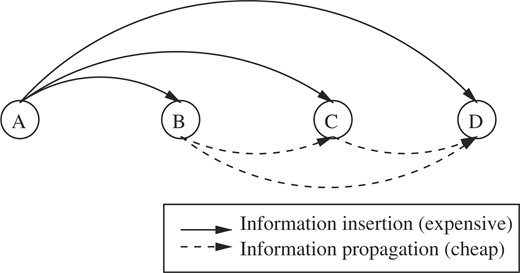
Generalization of the insert then propagate procedures to four decoys. A is the reference decoy. The distances AB, AC and AD are exactly measured while BC, CD and BD are easily approximated using ranges.
Hereafter, the formal definitions and algorithms previously introduced in prose are given.
2.2 Definitions and algorithms
Definition 1.
Neighborhood relation between decoys x and y at distance d: (x, y) ∈ {decoys}, d ∈ ℝ>0
neighbor(x, y, d) = ⊤ ⇔ rmsd(x, y) < = d
Definition 2.
Number of neighbors for decoy x from cluster c at distance d: d ∈ ℝ>0, c ∈ {clusters({decoys}, d)}, x ∈ c
nb_neighbors(x, c, d) = |{∀y ∈ c∣y ≠ x ∧ neighbor(x, y, d)}|
Definition 3.
Cluster center property for decoy x from cluster c: c ∈ {clusters({decoys}, d)}, (x, y) ∈ c
center(c, x) = ⊤ ⇔ ∄y∣(y ≠ x∧
nb_neighbors(y,c,d)>nb_neighbors(x,c,d))
Definition 4.
Decidability criterion for the decoy pair (x, y) at distance d: (x, y) ∈ {decoys}, d ∈ ℝ> 0
(rmsd(x, y) ∈ [rmin; rmax]) ∧ (0 <= rmin <= rmax)
decidable(x, y, d) ⇔ (rmin > d) ∨ (rmax <=d)
Definition 5.
Entropy for a set of decoys at distance d: (x, y) ∈ {decoys}, x≠y, d∈ℝ>0
entropy(d, {decoys}) = |(x, y)∣¬decidable(x, y, d):
It is interesting to note from Definition 3 that there can be several cluster center candidates, if they have an equal number of neighbors at cutoff distance d. The policy to choose the cluster center out of several equally ranked candidates is responsible for the instability of the algorithm. We refer to these equally possible cluster centers as ‘pole position centers’. Our implementation has a ‘stable’ option. It allows to display the pole position centers for the biggest cluster. Note that a cluster center in our definition is not a centroid (i.e. not an average of all the cluster members as is usually understood in the clustering literature). A cluster center in our approach is an actual cluster member (sometimes referred to as a ‘clustroid’), contrary to SPICKER which builds cluster representative structures by averaging all cluster members.
Our software implementation offers two ways to choose a cutoff value. The first method is directly via a user-specified value. The second method is semiautomatic. We used the latter during our experiments as it adapts automatically the threshold value to the spread of the decoy set, using a percentage parameter P provided by the user. In semiautomatic mode, Durandal will randomly sample pairwise RMSDs, and use the top P% sampled one as the cutoff value. The sample is grown iteratively by adding groups of 100 randomly chosen pairwise RMSDs out of the decoy set, to an initially empty set until the median of this set is stabilized.

3 RESULTS
3.1 Accuracy
To test the usefulness of our approach, we compared it against published results of SPICKER on I-TASSER decoys (Wu et al., 2007). We selected out of the full set 40 different protein targets. To be included in our study, a decoy set need to contain at least one good quality decoy (i.e. <4 Å CαRMSD to native). Each time, our software was run using semiautomatic threshold finding with P = 5% on the full decoy set (no shrinking applied). Results are shown in Figure 2. In each histogram, the first bar is the biggest cluster center discovered by Durandal while the second bar is the decoy nearest to the biggest cluster centroid computed by SPICKER [‘closc’ files in the decoy set from Wu et al. (2007)]. The best energy decoy as well as the nearest to native decoy from each set are shown as reference lines; clustering is useful only if it can pick decoys better than energy. We also tried P = 3% and P = 10% as the semiautomatic threshold finding parameter to verify the stability of our method. The maximal variation observed when using these different P-values in terms of average CαRMSD to native was only around 1.2%.
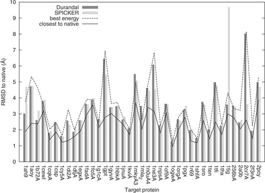
Clustering good-quality decoy sets from I-TASSER. The y-axis is the CαRMSD to the native structure. The x-axis is the protein sequence identifier used in I-TASSER, which is a combination of PDB code and chain letter. For each target, Durandal and SPICKER's choices are shown as histogram bars. The best energy decoy and the closest to native decoy in each set are shown as lines.
In our tests, in 25 out of 40 cases the biggest cluster center found by Durandal was nearer to native compared with the best energy decoy (20 out of 40 cases for SPICKER). On average, when comparing the chosen decoy from each method to the native structure, Durandal and SPICKER perform almost identically (3.35 Å CαRMSD and 3.37 Å CαRMSD, respectively).
3.2 Efficiency
Using geometric constraints propagation, our method allows to exploit efficiently the few CαRMSD that are computed during the insert-propagate phase (Fig. 3). Also, the speed of entropy decrease criterion allows to fall back to lazy completion at the optimal moment (Fig. 4).
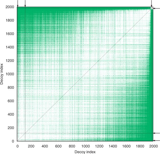
Colorized snapshot of the distance matrix after three insertion and three propagation steps (Algorithm 3). While having measured only 0.35% of all the possible CαRMSD pairs, our method completed 34.25% of the distance matrix initialization. White points are yet undecided decoy pairs. Green points are decided pairs that were estimated during propagation steps. Each black line is composed of decided pairs sharing the same reference decoy, exactly measured using CαRMSD during an insertion step. As the black lines from the three insertion steps plus their three symmetry mates are very thin, their positions are indicated by arrows at the upper and right sides of the picture. The black diagonal is the symmetry axis and also the not computed zero distance to self of each decoy. Decoys are sorted in the order of increasing CαRMSD to the decoy at index 0 for display purpose. The cutoff was 0.75 Å for 2k decoys of protein target 1aoy.
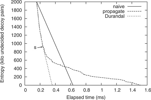
Different algorithms initializing the distance matrix at cutoff 0.75 Å on 2k decoys for protein target 1aoy. Entropy reaching zero is the terminating condition of the distance matrix initialization (a mandatory step prior to enumerating clusters). On the Durandal plot, the arrow labeled s indicates a switch in distance matrix initialization strategy from insert-propagate to lazy-completion (Algorithm 3).
In order to evaluate the speed gained with our method, we measured its execution times on some I-TASSER decoys while varying set size. We also tested our method on the ‘semfold’ decoy set (Samudrala and Levitt, 2002) (Downloaded from http://dd.compbio.washington.edu/). We compared elapsed times to that of Calibur, which is the fastest software we know that is capable of performing the same task. We also compared elapsed times to that of SCUD which is an approximate method. Calibur was extensively tested against SPICKER and shown to be significantly faster when working on large decoy sets (Li and Ng, 2010). Hence, we did not redo a comparison in speed with SPICKER.
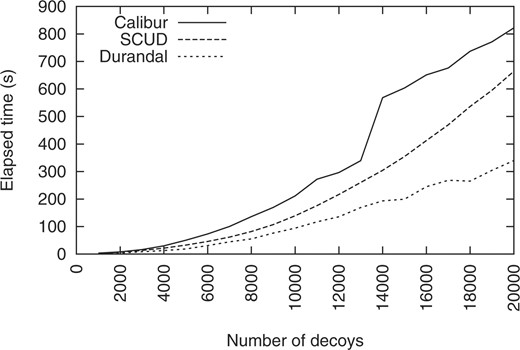
Speed comparison between Calibur, SCUD and Durandal on 1shfA decoys (1.5 Å cutoff). For clarity, only one slice in the 3D landscape created by varying the cutoff from 0.5 to 8 Å by 0.5 Å increment is shown. When considering the full cutoff range, Durandal is faster than Calibur in 98% of all cases. SCUD results were computed only for this slice.
All software were compiled using the highest optimization level (-O3) of their needed compiler. Durandal and Calibur are using the same routines to compute CαRMSD. All experiments were performed using exactly uniform computer cluster nodes. The PAR (Berenger et al., 2010) software (http://download.savannah.gnu.org/releases/par/par.tgz) was used to parallelize preparation of some input data, experiments, results analysis and obtain a shorter experiment turnaround with all softwares. On each dataset, every software was run five times with the same parameters. The averaged real-time elapsed as reported by the Linux ‘time’ command was retained. SCUD's run-time does

not vary as a function of the clustering threshold. However, the Calibur and Durandal run-times vary in a difficult to predict manner as a function of the clustering threshold and the distribution of decoys in the set. Durandal's run-time is also influenced by which references are used. All methods' speeds are influenced by the number of decoys in the set and the number of residues. Calibur was run without outlier filtering (to ensure exact clustering of the whole set is performed, as Durandal does). During Durandal runs, random reference selection was used to avoid input order bias. If references being used do not differ much from each other because they are chosen sequentially from the input files list and this list is somewhat ordered, it would penalize our algorithm. Results of comparison in speed with Calibur and SCUD while varying the decoy set size are shown in Figure 5. Accelerations observed on the ‘semfold’ decoy set are shown in Table 1. As a test to verify that both Calibur and Durandal implement correctly the exact clustering algorithm, some output files were randomly chosen and compared, showing a consistent 100% cluster similarity among the three biggest clusters (smaller clusters were not saved during experiments as Calibur outputs only top three by default).
Acceleration rate obtained by Durandal compared with SCUD and Calibur on the ‘semfold’ decoy set
| Target (decoys, residues) | Cutoff (Å) | SCUD | Calibur |
|---|---|---|---|
| 1pgb | 5 | 1.21 | 1.69 |
| (11 280, 56) | 6 | 0.9 | 1.49 |
| 7 | 0.75 | 1.61 | |
| 8 | 0.8 | 1.71 | |
| 1e68 | 4 | 2.08 | 1.75 |
| (11 361, 70) | 5 | 1.54 | 1.44 |
| 6 | 1.15 | 1.38 | |
| 7 | 0.95 | 1.61 | |
| 1ctf | 4 | 1.43 | 1.61 |
| (11 400, 68) | 5 | 1.38 | 1.57 |
| 6 | 1.08 | 1.47 | |
| 7 | 0.86 | 1.52 | |
| 1eh2 | 6 | 1.43 | 1.35 |
| (11 440, 95) | 7 | 1.01 | 1.06 |
| 8 | 0.85 | 1.28 | |
| 9 | 0.84 | 1.63 | |
| 1nkl | 5 | 1.73 | 1.42 |
| (11 660, 78) | 6 | 1.23 | 1.17 |
| 7 | 0.95 | 1.3 | |
| 8 | 0.81 | 1.51 | |
| 1khm | 5 | 1.99 | 3.22 |
| (21 080, 73) | 6 | 1.39 | 2.74 |
| 7 | 1.01 | 2.84 | |
| 8 | 0.85 | 3.4 |
The lower clustering threshold for each target was chosen so that the first cluster is statistically significant. Calibur and Durandal are exact methods while SCUD is approximate. The acceleration rates labeled ‘SCUD’ or ‘Calibur’ in the table are the total run-time of ‘SCUD’ or ‘Calibur’ divided by the total run-time of ‘Durandal’.
In Figure 5, the bump in Calibur run-times observed for set sizes larger than 13k decoys is due to a change of storage data structure at run-time (a default Calibur behavior that the user has no control over). In Figure 5, the average acceleration rate obtained by Durandal compared with Calibur is 2.53 and 1.74 compared with SCUD. In Table 1, our method is shown to be consistently faster than Calibur and can even outperform SCUD in some cases.
4 DISCUSSION
Distance matrix computation is the most time consuming part of exact clustering. It is interesting to look at how the same problem was approached in two different ways by Calibur and Durandal. Calibur's algorithm grows clusters stepwise in an online manner. Calibur's focus is targeted at grouping together proximate decoys so the problem is looked from a spatial organization viewpoint. Durandal computes clusters off-line, once enough information is known regarding distances of all decoy pairs. Distance information are inserted into the distance matrix using methods to maximize the speed of the procedure. Durandal attacks the problem using an information-centered approach. One of the consequences of these different strategies is that Calibur does not fully exploit some of the expensive methods to compute information it collects. In Calibur, some previously computed distances or their bounds are used to avoid computing some more distances, but this information does not percolate through all clusters. Whereas in Durandal, as long as inserting then propagating new distance information is the fastest strategy, information is exploited to the maximum.
Both SPICKER and Durandal implement the same clustering algorithm. However, some slight differences remain. Both methods use different automatic threshold-finding strategies, decoy selection technique and energy filtering. Concerning threshold-finding strategy, SPICKER follows a cutoff refinement algorithm (Zhang and Skolnick, 2004a) while Durandal picks a value after some quick sampling of the decoy set. Durandal's way is close to Calibur's default threshold-finding strategy. For decoy selection, SPICKER selects the decoy nearest to the cluster centroid while Durandal selects the cluster center as understood in Definition 3. Moreover, Durandal clusters full decoy sets without applying additional energy filtering, whereas SPICKER reduces the decoy set to 13k decoys maximum using an energy criterion. When the energy function is inaccurate, Durandal may benefit more from the averaging effect of clustering.
We have addressed the problem of clustering speed to a large extent with Durandal. However, the memory requirement issue has not been dealt with. The memory requirement grows in the same order as that of the naive algorithm. This is an important problem. Clustering acceleration can be tackled using geometric constraints as we did. If the distance measure being used is not a metric, our approach cannot be applied to speed up the process by reducing the number of calls to the distance function. The memory problem is not easy to address; if the distance matrix were stored on disk, the overall clustering procedure would become an order of magnitude slower due to the higher disk access latency compared with memory. Algorithms avoiding the memory size problem should work under the constraint: being able to cluster without requiring that the full distance matrix is available in memory. In this aspect, despite Calibur's speed being far from optimal, it is worthwhile noticing that it is quite thrifty regarding memory consumption.
Concerning the optimum choice of reference decoys in Durandal, previous work employing a metric distance in the problem of best-match search showed that there is an optimal heuristic to choose reference points (Shapiro, 1977). Reference points should be away from cluster centers. However, the exact distance away, as well as the number of reference points to use is unclear. Concerning the number of references to consider, our algorithm uses an entropy decrease speed criterion to detect if we are starting to use too many of them in order to trigger a fallback from the insert-propagate step to the lazy-completion one. Durandal uses chance in its reference point choice policy. Based on our experience using Durandal, the speed criterion combined with random reference selection creates an efficient and simple heuristic.
Some distributed algorithm could push even further the scalability of clustering large decoy sets, both in terms of speed and memory requirements. In the distributed case, the problem would probably be no longer just about fast clustering where our algorithm could be used. The challenge may become how to efficiently merge and store intermediate clustering results from partitions of a whole decoy set. Possibly, some small overlapping in the partitions could accelerate the procedure by merging first reference structures from both sets. Afterwards, many distance measures would be avoided. If the user is not interested in parallelizing computations, the parallel version of the program could still be used to overcome the memory barrier by running it sequentially on a single computer. Partitioning the initial set, and then clustering each subset before incrementally merging results seems a feasible approach.
We hope the method we proposed will help the protein folding community in the decoy identification step of their protocols. The acceleration technique we detailed may be of interest to other scientific or engineering fields and may be adapted to other clustering algorithms.
1In the rest of this article and unless otherwise mentioned, RMSD always means Root-Mean-Square Distance after optimal superposition. CαRMSD stands for RMSD considering only Cα atoms.
2URMSD stands for unit-vector RMSD. It is a non protein-length biased version of the popular CαRMSD (Kedem et al., 1999).
3Sometimes referred to as ‘clustering threshold’ or even ‘cluster cutoff’.
ACKNOWLEDGEMENTS
We wish to thank RIKEN, Japan, for an allocation of computing resources on the RIKEN Integrated Cluster of Clusters (RICC) system. We are largely indebted to protein folding researchers who make publicly available full decoy sets.
Funding: Initiative Research Unit program from RIKEN, Japan.
Conflict of Interest: none declared.
REFERENCES
Author notes
Associate Editor: Anna Tramontano

