


Abstract
Motivation: Many ChIP-Seq experiments are aimed at developing gold standards for determining the locations of various genomic features such as transcription start or transcription factor binding sites on the whole genome. Many such pioneering experiments lack rigorous testing methods and adequate ‘gold standard’ annotations to compare against as they themselves are the most reliable source of empirical data available. To overcome this problem, we propose a self-consistency test whereby a dataset is tested against itself. It relies on a supervised machine learning style protocol for in silico annotation of a genome and accuracy estimation to guarantee, at least, self-consistency.
Results: The main results use a novel performance metric (a calibrated precision) in order to assess and compare the robustness of the proposed supervised learning method across different test sets. As a proof of principle, we applied the whole protocol to two recent ChIP-Seq ENCODE datasets of STAT1 and Pol-II binding sites. STAT1 is benchmarked against in silico detection of binding sites using available position weight matrices. Pol-II, the main focus of this paper, is benchmarked against 17 algorithms for the closely related and well-studied problem of in silico transcription start site (TSS) prediction. Our results also demonstrate the feasibility of in silico genome annotation extension with encouraging results from a small portion of annotated genome to the remainder.
Availability: Available from http://www.genomics.csse.unimelb.edu.au/gat.
Contact: [email protected]; [email protected]
Supplementary Information: Supplementary data are available at Bioinformatics online.
1 INTRODUCTION
The recent advances in microarray technologies (tiling arrays, SNP arrays, etc.) and more recently in high-throughput sequencing [next-generation sequencing (NGS)] allows for more complete genome-wide annotation of functional sites. The rapid increase in the data volumes has put pressure on the development of data analysis techniques capable of coping with large volumes of data that can reliably extract relevant knowledge. This article analyses and benchmarks techniques introduced in Kowalczyk et al. (2010) based on supervised learning and the generalization capabilities of predictive models that are trained on part of the genome and tested on the remainder. Our approach consists of dividing the genome into small tiles and then allocating a binary label to each tile according to the observed phenomenon (e.g. the presence of a transcription factor binding site within the tile). A model is then trained on a portion of the genome to predict the labels from the DNA content of tiles and then tested on the whole genome. The prediction accuracy is then used to assess the properties of the assay.
There are many interesting phenomena which can be analysed by this approach and we will now focus on two key examples:
A quality test for ChIP-Seq experiment: we first discuss a quality test for ChIP-Seq experiments when there is no (independent) gold standard to assess the final results. In the paper by Kowalczyk et al. (2010), we compared a few sets of putative peaks for STAT1 and Pol-II binding sites generated by various analysis methods applied to the ChIP-Seq experimental data of Rozowsky et al. (2009). As the ‘gold standards’ provided by the ENCODE project were extracted from the same experimental data and their putative peaks were a part of our comparative study, an independent and objective way of evaluating the various lists of peaks was required.
Kowalczyk et al. (2010) introduced a consistency benchmark: for each list of putative peaks ordered by the allocated P-values, a model was trained using only chromosome 22 to predict the overlap of a tile with a peak from the tile's DNA content. The model was then applied to the whole genome and its predictions compared with the list of putative peaks. The lists, and the peak calling algorithms generating them, that provided more consistent (accurate) predictions deemed to be more accurate. Significant differences in the peak calling algorithms were observed. The article is linked directly to those methods developed by Kowalczyk et al. (2010), for both Pol-II and STAT1, but here the focus is mainly on predicting Pol-II.
An extension of annotation: a critical hurdle in the way to full ‘mechanistic’ interpretation of genetic data is extending the annotation of the human genome such that every regulatory sequence in the genome is identified along with known disease-associated genetic variations and changes. The analysis of the transcriptome by NGS methods generates novel genomic expression landscapes, state-specific expression, single-nucleotide polymorphisms (SNPs), the transcriptional activity of repeat elements and both known and new alternative splicing events. These all have an impact on current models of key signalling pathways ‘... suggesting that our understanding of transcriptional complexity is far from complete’ (Cloonan et al., 2008). In particular, as transcripts are often state and cell type specific, the proper annotation of gene boundaries is compromised until all the conditions of all cells are properly profiled—a formidable molecular task. Moreover, as NGS is relatively recent many cell states and types have been profiled on tiling arrays or standard gene expression arrays covering only a relatively small part of the human genome and have not been analysed genome-wide using NGS. Thus, there is immediate benefit in developing tools that would extend key regulatory element mapping, such as the binding of STAT1 or transcriptional start sites, from a fraction of the genome where it was empirically explored, either using promoter arrays (Affymetrix, Nimblegen, etc.) or with ENCODE tools, through to the whole genome.
Implementation of the above ideas rests on the assumption that robust and simple predictive models can be developed and their performance can be meaningfully measured against annotations with extreme class imbalances, where the positive classes are very sparse (which is the typical case for most genome functional annotations). The aim of this article is to demonstrate that such solutions are feasible and applicable to NGS genome-wide studies of current interest.
The whole method depends critically on the generalization capabilities of a supervised learning predictor. To that end, we mainly focus on the performance of our method for predicting Pol-II binding and on the closely related task of (in silico) transcription start sites (TSS) prediction. This annotation (rather than STAT1) was chosen as it is well studied with high-quality data and in silico prediction results are readily available. A recent extensive comparative study of TSS in humans (Abeel et al., 2009) has demonstrated that supervised learning techniques performed the best, with the SVM-based predictor ARTS (Sonnenburg et al., 2006) being the clear winner. We demonstrate a successful technique with performance equivalent to ARTS at the coarse 500 bp resolution, but with much simpler training. As our method uses only a handful of generic features (k-mer frequencies) in a linear fashion,1 it is also more universal. In order to demonstrate the generalization capabilities convincingly, we have used only data from the smallest autosomal human chromosome (chromosome 22, ~ 1/60th of the genome) for training, which is typically much less than the size of the active genome in a ChIP-Seq experiment. Chromosome 22 is often used for incomplete annotation experiments on the human genome (Hartman et al., 2005).
The algorithmic details and the formal derivation of the key metric (calibrated precision) can be found in the Supplementary Materials.
2 GENOME ANNOTATION METHODOLOGY
We now outline the principles of the proposed methodology for genome annotation and the methods for measuring the performance. Technical details are available in the Supplementary Material.
2.1 Genome segmentation
The genome was segmented into overlapping 500 bp tiles, shifted every 250 bp. Thus, each nucleotide is covered by exactly two tiles. Overlapping tiles are used to mitigate the effect of edges; for each nucleotide, the 250 bp neighbourhood centred around the nucleotide is fully contained in exactly one 500 bp tile. Thus, the whole human genome is composed of 10.72M different tiles. We have also analysed a reduced dataset containing 0.96M tiles (see Table 1, Column ‘RefGeneEx’). Each dataset has its own set of binary labels yi= ±1 allocated to each tile  , see Section 3.1 for details.
Dataset summary
| Label set | Pol-II | RefGene | RefGeneEx |
|---|---|---|---|
| Training sets for RSV(= intersections with chromosome 22) | |||
| n+ | 3.2K | 1.0K | 1.0K |
| n− | 140K | 140K | 12K |
| Test sets | |||
| n+ | 160K | 43K | 43K |
| n− | 11M | 11M | 0.55M |
| n+/(n++n−) | 0.015 | 0.0039 | 0.072 |
| Label set | Pol-II | RefGene | RefGeneEx |
|---|---|---|---|
| Training sets for RSV(= intersections with chromosome 22) | |||
| n+ | 3.2K | 1.0K | 1.0K |
| n− | 140K | 140K | 12K |
| Test sets | |||
| n+ | 160K | 43K | 43K |
| n− | 11M | 11M | 0.55M |
| n+/(n++n−) | 0.015 | 0.0039 | 0.072 |
2.2 Feature extraction
For each tile the features for learning and classification were generated from its DNA content exclusively as the occurrence frequencies of k-mers. Previously, we have experimented with a few variations of the method, including different values of k (Bedo et al., 2009; Kowalczyk et al., 2010). For this article, we exclusively used k = 4 and also combined the frequencies for forward and reverse complement pairs; such a summation simplifies the models with a marginal difference in performance. Furthermore, for notational convenience (see the next section) we add a constant feature of value 1. Thus, the feature vector function  maps each tile into a
  -dimensional space.
2.3 Supervised learning
We used a simple linear classifier in the feature space defined above:

where  . The weight vector
  was obtained using a support vector machine combined with recursive feature elimination. Typically, only a fraction of features are used – i.e. they have weights wi≠ 0. The algorithm is referred to as a recursive support vector (RSV) machine and is described in Section 1 of the Supplementary Material.
2.4 Performance metrics

and the precision is
where nr: = n+r+ n−r and n+ and n− denote the total number of positive and negative examples, respectively. The precision–recall curve (PR curve or PRC) is simply the plot of the precision versus recall, as defined above. The area under the PRC (auPRC) is used as a general measure of performance across all thresholds (Abeel et al., 2009; Sonnenburg et al., 2006).
The second classical metric considered here is centred on the receiver operating characteristic (ROC) curve and the area under it (auROC) (Hanley and McNeil, 1982). This is a well-established performance measure in machine learning, bioinformatics and statistics.
We define the ROC curve as the plot of the specificity
versus the recall. Note that this curve is clockwise-rotated 90° with respect to the typical ROC curve used by the machine learning community. The auROC has been shown to be equivalent to the probability of correctly ordering class pairs (Hanley and McNeil, 1982).
2.4.1 Calibrated precision–recall
The PRC and ROC curve are typically used for comparing performance of predictors on a fixed benchmark. However, when one evaluates a novel ChIP-Seq experiment—see for example the Pol-II benchmark below—there is no other predictor or dataset to compare performance against. Thus, a form of ‘calibration’ is needed to evaluate the predictor performance in isolation to determine if a sufficient generalization level is achieved.
Example 2.1
Let us consider two test datasets with radically different positive samples prior probability: (A) n+/(n+ + n −) = 5% and (B) n+/(n+ + n −) = 95%. If we use a uniformly random classifier, its expected precision at any recall level will be 5% in case A and 95% in case B. Now, consider two non-random predictors: fA with precision p = 10% on set A and fB with precision p = 99% on set B, both at recall ρ = 20%. Which of them performs better? The question is not straightforward to resolve. On the one hand, the predictor fA performs two times better than random guessing, while fB performs only 1.04 times better than random guessing. Thus, in terms of the ratio to the expected performance of a random classifier, fA performs far better than fB. However, in case A the perfect predictor is capable of 100% precision—i.e. 10× better than random guessing and 5× better than fA—while in case B, the perfect predictor is capable of only 1.05× better than random guessing. This is approximately what fB is capable of, so fB now seems stronger than fA!
To resolve this problem, rather than analysing ratios as in the above example, we can ask a different question: what is the probability of observing a precision better than random guessing at a given recall? The smaller such a probability, the better the performance of the classifier, hence it is convenient to consider − log10 of those probabilities. We call this the calibrated precision (CP); better classifiers will result in higher values of CP. The plot of CP as a function of recall is referred to as the calibrated precision–recall curve (CPRC). The explicit formula for CP is2:
This formula explicitly depends on values of n+ and n−, thus different results are expected for different class sizes even if their ratio is preserved. Indeed, if we assume n = n++ n−= 103, then the respective values of the calibrated precision for Example 2.1 are CPA= 3.74 and CPB= 4.85, while for n = 106 we get CPA= 904.3 and CPB= 2069.2. This is a trend which one should expect: intuitively, dealing with datasets containing hundreds of examples is far easier than dealing with dataset containing millions. More formally, in the latter case although we have the same proportion of correct guesses—i.e. the same precision at the same recall level—the absolute number of correct guesses is proportionally higher. This is much harder due to the central limit theorem of statistics as the average of a larger number of repeated samplings has a stronger tendency to converge to the mean with a variance inversely proportional to the number of trials. Thus, for larger datasets the same deviation from the mean is associated with a far smaller probability of occurrence. The above simple example vividly illustrates this principle, which is also clearly visible in the empirical test results in Figure 2B and Table 3.
As usual it is convenient to convert CPRC into a single number for easy comparisons. We use two options here: the maximal rise of CPRC [max(CP) : = maxρCP(p(ρ), ρ)] and the area under the CPRC (auCPRC). The latter option is in line with areas under ROC and PRC and can be interpreted as the expected CP on the space of positively labelled test examples (see the Section 3 of Supplementary Material).
Remark 2.1.
One simple method for compensating for the differences in test sets could be to calibrate the precision–recall curve by dividing it by the prior probability of the positive labels [this is the concept of precision enrichment (PE) and is discussed more in Section 5 of the Supplementary Material]. However, this may be a very bad solution if the test set sizes are different.
To clarify the point, let us consider the following two extreme examples:
A. a trivial case with n+= 2 and n−= 18, and
B. a non-trivial case with n+= 200K and n−= 9 × 10⁶ examples.
In both cases, let us consider predictors achieving precision p = 50% at recall of ρ = 50%. Which predictor performs better? The priors of the positive classes are 10 and 20%, respectively, hence PEA(50%) = 5 > PEB(50%) = 2.5 indicating A is the superior predictor. However, with a uniform random shuffling of the data, we achieve precision (pA ≥ 50%) ≡ (PEA ≥ 5) at p = 50% with probability > 25%, while the analogous probability for pB ≥ 50% and (PEB > 2.5) ≡ (p = 50%) is ≤ CP~ 10 − 97408. Thus, the performance of B, being practically impossible to match or improve by chance, is superior.
3 RESULTS
In Section 3.1–3.4 below, we cover the main experiments with detection of Pol-II binding and in silico TSS detection. In Section 3.5, we outline additional experiments with ChIP-Seq data for transcription factor STAT1.
3.1 Datasets for Pol-II and TSS
We used five different datasets for training and testing our classifiers. The first two were whole genome scans while the third was designed to be similar to the benchmark tests used by Abeel et al. (2009) and Sonnenburg et al. (2006); the last two are independent benchmark sets embedded in the software of Abeel et al. (2009).
Pol-II: this is our main benchmark. The recent ChIP-Seq experimental data of Rozowsky et al. (2009) provides a list of 24 738 DNA ranges of putative Pol-II binding sites for the HeLa cell line. These ranges are defined by a start and end nucleotide. The lengths are varying between 1 and 74 668 and have a median width of 925 bp. Every 500 bp tile (as described in Section 2.1) was given label 1 if overlapping a range and − 1 otherwise. This provided ~ 160K positive and ~ 11M negative labels.
RefGene: for this dataset, we have used human reference genome hg18 with RefGene annotations for transcribed DNA available through the UCSC browser. It annotates ~32K TSSs including alternative gene transcriptions. More specifically, if a 500 bp tile was overlapping the first base of the first exon it was labelled +1, and if not it was labelled − 1. This created n+= 43K positive and n−= 11M negative examples.
RefGeneEx: this is an adaptation of the previous dataset to the methodology proposed by (Sonnenburg et al., 2006) and adopted by Abeel et al. (2009) in an attempt to generate more reliable negative labels. The difference is that all negative examples that do not overlap at least one gene exon are discarded. This gives n+= 43K positive and only n−= 0.55M negative examples.
3.2 Predictors
We used three different RSV predictors for Pol-II and TSS experiments, namely RSVPo2, RSVRfG and RSVEx, each trained on the intersection of chromosome 22 with one of the above datasets using the method described in Section 2.3 (with details in Section 1 of the Supplementary Material).
The predictions for ARTS were downloaded (http://www.fml.tuebingen.mpg.de/raetsch/suppl/arts/) from a web site published by the authors of the algorithm (Sonnenburg et al., 2006). These predictions contain scores for every 50 bp segment aligned against hg17. The liftOver tool (http://hgdownload.cse.ucsc.edu/goldenPath/hg17/liftOver/) was used to shift the scores to hg18. For the results reported in Figures 1 and 2, and Table 3, we took the maximum of the scores for all 50 bp tiles contained within each 500 bp tile as in Section 2.1.
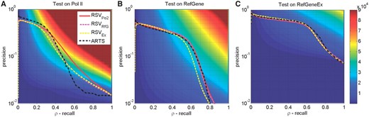
Comparison of the PRCs grouped by test sets, with subfigures ordered in the descending order of (n+, n−)-sizes: (A) for Pol-II (Rozowsky et al., 2009), (B) RefSeq TSS database and (C) RefSeqEx databases; see Table 1 for summary and Section 3.1 for details. We plot the PRCs for four different predictors as in Section 3.2. The background shading shows calibrated precision, CP(prec, recall), see (4); values in (A) and (B) are clipped at maximum 9×10⁴ for better visualization across all figures (we use the same colour scale across them).
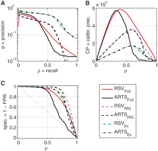
Comparison of three methods of evaluation for six different predictors: three versions of RSV developed as specified in Table 3 and ARTS tested on three datasets, as indicated by subscripts. (A) PRC; (B) CPRC; (C) ROC curves.
The training datasets for RSV predictors are summarized in Table 1. They are overlaps of the respective label sets with chromosome 22 only. In contrast, ARTS used carefully selected RefGene-annotated regions for hg16. This resulted in n+= 8.5K and n−= 85K examples for training, which contain roughly 2.5–8 times more positive examples than used to train our RSV models. Additionally, the negative examples for ARTS training were carefully chosen, while we have chosen all non-positive examples on chromosome 22 for RSV training, believing that the statistical noise will be mitigated by the robustness of the training algorithm.
3.3 Benchmark against 17 promoter prediction tools
Our three predictors, RSVPo2, RSVRfG and RSVEx generated as described in Section 3.2, were compared against 17 dedicated promoter prediction algorithms evaluated by Abeel et al. (2009) using the software provided by the authors. This software implements four different protocols:
1A: Bin-based validation using the (preprocessed) CAGE dataset3 as a reference. This protocol uses non-overlapping 500 bp tiles, with positive labels for tiles that overlap the centre of the transcription start site and negative labels for all remaining tiles.
1B: this protocol is similar to 1A except it uses the RefGene set as a reference instead of CAGE. The tiles overlapping the start of the gene are labelled +1, the tiles that overlap the gene but not the gene start are labelled − 1 and the remaining tiles are discarded.
2A: this is a distance-based validation with the (pre-clustered) CAGE dataset as a reference. A prediction is deemed correct if it is within 500 bp from one of the 180 413 clusters obtained by grouping 4 874 272 CAGE tags (Section 2.1Abeel et al., 2009). For this and the following test, we have associated the RSV prediction for every tile with the centre of the tile, which is obviously suboptimal.
2B: according to Abeel et al. (2009): ‘this is a modification of protocol 2A to check the agreement between transcription start region (TSR) predictions and gene annotation. This method resembles the method used in the EGASP pilot-project (Bajic et al., 2006).’
The results are summarized in Table 2, where we compare them to a subset of top performers reported by (Table 2Abeel et al., 2009). Only 1 of the 17 dedicated algorithms they evaluated—the supervised learning-based ARTS—performed better then our classifiers in terms of overall PPP score [the harmonic mean of four individual scores for tests 1A-2B introduced in Abeel et al. (2009)], and only three additional algorithms have shown performance better or equal to our predictors on any individual test. This is unexpected as those dedicated algorithms used a lot of special information other than the local raw DNA sequence; some of which were developed using carefully selected positive and negative examples covering the whole genome rather than only a small subset of it, as in the case of our RSV training.
Results of testing our predictors using the four benchmarks protocols of Abeel et al. (2009) and then comparing against 17 algorithms they evaluated.
| Name | 1A | 1B | 2A | 2B | PPP score |
|---|---|---|---|---|---|
| Our results using software of Abeel et al. (2009) | |||||
| RSVPo2 | 0.18 | 0.28 | 0.42 | 0.55 | 0.30 |
| RSVRfG | 0.18 | 0.28 | 0.41 | 0.56 | 0.30 |
| RSVEx | 0.18 | 0.28 | 0.41 | 0.56 | 0.30 |
| Results in Abeel et al. (2009) with performance ≥ any RSV | |||||
| ARTS | 0.19 | 0.36 | 0.47 | 0.64 | 0.34 |
| ProSOM | 0.18 | 0.25 | 0.42 | 0.51 | 0.29 |
| EP3 | 0.18 | 0.23 | 0.42 | 0.51 | 0.28 |
| Eponine | 0.14 | 0.29 | 0.41 | 0.57 | 0.27 |
We show the results for ProSOM (Abeel et al., 2008a), EP3 (Abeel et al., 2008b), Eponine (Down and Hubbard, 2002) and ARTS. The results are sorted according to the PPP score, which is the harmonic mean of the four individual scores giving an overall figure of merit. All results better than our ChIP-Seq developed model RSVPo2 are marked in bold face; apart from ARTS there are only the two such results, both with the Eponine algorithm. The results for the remaining 13 algorithms have worse performance than every RSV for tests 1A–2B and can be found in Table 2Abeel et al. (2009).
3.4 Self-consistency tests
The PR curves for all four predictors on three datasets are shown in Figure 1. The subplots A and B show results for the genome-wide tests on Pol-II (Rozowsky et al., 2009) and RefSeq database, respectively, while the third subplot, C, uses the restricted dataset RefSeqEx (covering ~ 1/20 of the genome). The PRC curves on each subplot are very close to each other. Thus, RSVPo2, RSVRfG, RSVEx and also ARTS show very similar performance on all benchmarks despite being trained on different datasets. However, there are significant differences in those curves across different testsets, with the curves for subplot C being much higher with visibly larger areas under them than for the other two cases—i.e. for the genome-wide tests. However, this does not translate to statistical significance. The background colour shows stratification of the precision–recall plane according to statistical significance—i.e. the calibrated precision CP(p, ρ) defined by (4)—for which we have used the same colour scheme on all figures. We observe that curves in subplot A run over much more significant regions (closer to red) than the curves in C, with B falling in between. This is due to the following: in case A, we are detecting n+~ 160K samples in the background n−~ 11M samples. Thus, it is much harder task to achieve a particular level of precision for a particular recall than in case C, which deals with ‘only’ one-quarter of the positive samples, n+~ 43K, embedded into the 20-times smaller background of n−~ 550K negative cases.
Note also that the most significant loci are different from the loci with the highest precision. In terms of Figure 1A and the RSVPo2 predictor, it means that the precision p~ 58.2% achieved at recall ρ~ 1% with CP ~ 2.1K is far less significant than p ~ 25% achieved at ρ ~ 38%, which reaches a staggering CP ~ 58.4K.
To further quantify impact of the test data—i.e. the differences between genome-wide analysis and restriction to the exonic regions—we have combined in Figure 2 the different benchmark sets for which we have evaluated the three metrics PRC, ROC and CPRC. The main difference between Figures 1 and 2 is that, for clarity, in the latter figure we show for each RSV predictor the genome-wide test results only for annotations used in the training the predictor (on chromosome 22)—i.e. we do not show cross-dataset testing results as in Figure 1.
In Figure 2A, we observe that PRC for RefGeneEx clearly dominates the other curves. The curves for RSVPo2 and ARTSPo2 seem to be much poorer, which is supported by the ROC curves in Figure 2C. However, the plots of CPRC in Figure 2B tell a completely different story. The differences shown by the colour shadings in Figure 1 are now translated into the set of curves which clearly differentiate between the different test benchmark sets, allocating higher significance to the more challenging benchmarks.
Some of those differences are also captured numerically in Table 3. We list here the area under the curves, auPRC, auCPRC and auROC, as well as the maximum calibrated precision max(CP) with the corresponding values of precision and recall. We list values for RSV classifiers and corresponding tests for ARTS. The most significant values are shown in boldface. The performance of RSV and ARTS are remarkably close, with ARTS slightly prevailing on the smallest test set RefGeneEx, which is the closest to the training set used for ARTS training, while RSV predictors are better on the two genome-wide benchmarks. However, those difference are minor, with the most striking observation being that all the classifiers are performing so well in spite of so many differences in their development. This should be viewed as a success for supervised learning which could robustly capture information hidden in the data (in a tiny fraction, 1/60th of the genome in the case of RSV).
Numerical summary of the performance curves for the six predictors compared in Figure 2.
| Metric | Pol-II (Po2) | RefGene (RfG) | RefGeneEx (Ex) |
|---|---|---|---|
| auPRC | 0.22/0.22 | 0.23/0.22 | 0.47/0.46 |
| auCPRC | 34K/23K | 19K/18K | 9.0K/9.3K |
| auROC | 0.81/0.69 | 0.88/0.84 | 0.82/0.83 |
| max(CP) | 58.4K/57.2K | 36.0K/35.6K | 17.2K/17.5K |
| Arguments of max(CP) | |||
| Precision | 0.25/0.31 | 0.20/0.20 | 0.51/0.48 |
| Recall | 0.38/0.24 | 0.59/0.57 | 0.57/0.60 |
| n+r | 61K/54K | 24.3K/24.1K | 24.1K/25.3K |
| nr | 243K/177K | 123K/120K | 47K/53K |
| n | 10.7M | 10.7M | 0.59M |
The auPRC, auCPRC and auROC denote the areas under the PRC, CPRC and ROC curves in Figure 2A, C & D, in the format RSVdataSet/ARTSdataSet, respectively. We show also max(CP), see (4) with the corresponding values of the arguments, i.e. precision and recall.
We observe that max(CP) is achieved by RSVPo2 for precision 25% and recall 38% positive samples out of n+ = 160K. This corresponds to compressing n+r= 61K target patterns into the top-scored nr= 243K samples out of n = 10.7M. In comparison, the top CP results for ARTS on RefGeneEx data resulted in compression of n+r= 25.3K of positive samples into the top scored nr= 47K out of a total of n = 0.59M. Note that in the test on RefGene the results are more impressive than for RefGeneEx: roughly the same number of positive samples n+= 23.4K was pushed into the top nr= 123K out of a total of n = 10.6M, which is ~ 20 time larger.
Note that Figure 2C shows that ROC is not discriminating well between performance of different predictors in the critical regimes of the highest precision, which inevitably occurs for low recall (ρ < 0.5). Thus, ROC and auROC have a limited utility in the genome-wide scans with highly unbalanced class sizes.
Note also that the better precision at low recall shown by ARTSPo2 compared with RSVPo2 in Figure 1A, Figure 2A and Figure 2C did not translate to significantly better CP in Figure 2B. The better performance of RSVPo2 for higher recall has turned out to be much more significant resulting in higher auCPRC in Table 3. It is worth noting that the results for RSVPo2 and ARTSPo2 are not completely comparable as ARTS was trained on RefGene and not on the Pol-II labels and used more information, but was specifically aimed at the finer 50 bp resolution. Training ARTS on the Pol-II labels is not straightforward as the spatial structure of the DNA is not readily available and many Pol-II peaks are very wide, lacking the precision of RefGene TSS location.
3.5 A control experiment for STAT1
As we have stated already, the application of RSV predictors to assess different peak calling routines for STAT1 ChIP-Seq data [ENCODE data, published by Rozowsky et al. (2009)] was presented by Kowalczyk et al. (2010), with a few small differences: Kowalczyk et al. (2010) used non-overlapping tiles, the analysis was based purely on (un-calibrated) PRCs and peaks other than those identified in Rozowsky et al. (2009) were used. In contrast in this article, we use only the original peak calls of Rozowsky et al. (2009) for training our predictor RSVSTAT1 on chromosome 22 followed by testing on the whole genome. We also compare its performance against a number of position weight matrices (PWM) available for STAT1 from the TRANSFAC and JASPAR databases. Thus, our main novel contribution is the quantification of the performance of RSVSTAT1 in terms of CPR and benchmarking against the PWMs. Note that the global scans by PWMs, as well as the detection of ‘weakly-binding’ sites, are of direct interest for in silico cis-regulatory module detection, so in this context the performance assessment of predictive models outside of the highest precision peaks is important.
The ChIP-Seq dataset of Rozowsky et al. (2009) for STAT1 consists of 36 998 peaks of varying sizes, between 1 bp and 86 514 bp with median 425 bp. Similar plots to those shown previously for RSVSTAT1 are shown in Figure 3. For a PWM scan, we allocated to each 500 bp tile the maximal score achieved by sliding the PWM over each base. We see that RSVSTAT1 dominates all PWMs apart from a few highly accurate peaks, which turned out to be statistically insignificant due to small recall (see CPRC plots in Figure 3B). This indicates that some PWMs are highly tuned to some small subclasses of binding sites, while RSV is capable of learning more global characteristics. Note, the performance of some PWMs is on the level of random ordering.
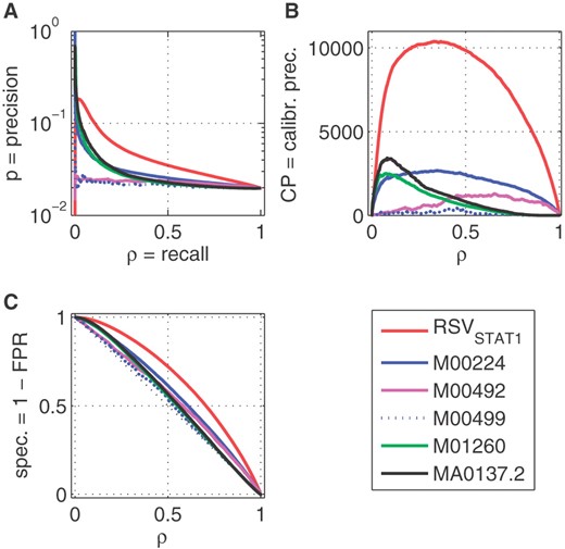
Comparison of RSVSTAT1 and six scans of human DNA using different PWMs for STAT1 (M00224, M00492, M00496 and M01260 from TRANSFAC and MA0137.2 from JASPAR databases). (A) PRC; (B) CPRC; (C) ROC curves. There are n+= 211K positive and n−= 10.5M negative tiles in this case and the expected precision for random guessing is ~ 2% which is approximately the level for some PWMs in subplot A. A numerical summary is presented in Supplementary Table S2.
4 DISCUSSION
In this article, we aimed to demonstrate that ChIP-Seq results can be used to develop robust predictors by training on a small part of the annotated genome and then testing on the remainder, primarily for the purpose of cross-checking the consistency of the ChIP-Seq results and also for novel genome annotation. As a proof of principle, we have chosen two ENCODE ChIP-Seq datasets for binding of the transcription factor STAT1 and the Pol-II complex. STAT1 experiments have shown that RSV models are superior in learning global patterns compared with standard PWM-based approaches.
For Pol-II, where PWMs are not applicable, we have compared against the best-of-class in silico TSS predictors ARTS as TSS is closely related to Pol-II binding. Though ARTS is our focus as a baseline, we also benchmarked against 16 other specialized algorithms using the methods of Abeel et al. (2009). Our predictors are created by a generic algorithm and not a TSS specific procedure with customized problem-specific input features; for instance, we do not take into account the directionality of the strands, which may improve performance, as such information is not available from empirical ChIP-Seq data. Nevertheless, we have demonstrated that the lack of such information does not prevent the development of accurate classifiers on-par with dedicated tools such as ARTS at the 500 bp resolution.
For our aim of developing a generic and robust technique for genome annotation, ARTS, originally intended for higher 50 bp resolution, is too specialized and overly complex; indeed, ARTS uses five different sophisticated kernels—i.e. custom-developed techniques for feature extraction from DNA neighbourhood of ± 1000 bp around the site of interest. This includes two spectrum kernels comparing the k-mer composition of DNA upstream (the promoter region) and down stream of the TSS, the complicated weighted degree kernel to evaluate the neighbouring DNA composition, and two kernels capturing the spatial DNA configuration (twisting angles and stacking energies). Consequently, ARTS is very costly to train and run: it takes ~ 350 CPU hours (Sec. 3.1Sonnenburg et al., 2006) to train and scan the whole genome. Furthermore, for training the labels are very carefully chosen and cross-checked in order to avoid misleading clues (Sec. 4.1 Sonnenburg et al., 2006).
In contrast, our generic approach is intended to be applied to novel and less-studied DNA properties, thus we do not assume the availability of prior knowledge. Consequently, our model uses only standard and generic genomic features and all available labelled examples in the training set. It uses only a 137-dimensional, 4mer-based vector of frequencies in a single 500 bp tile, which is further simplified using feature selection to ~ 80 dimensions. This approach is generic and the training and evaluation is accomplished within 4 CPU hours (Bedo et al., 2009).
The success of such a simple model is surprising and one may hypothesize about the reasons:
Robust training procedure: this includes the primal descent SVM training and using auPRC rather than auROC as the objective function for model selection;
Simple, low dimensional feature vector;
Feature selection/reduction.
We stress again that as stated in Section 3.1, for the sake of fairness, we have used not only ChIP-Seq trained RSV models, but also two different models RSVRfG and RSVEx, which are trained using RefGene annotations only, which were used for training ARTS. However, while ARTS used all RefGene annotations available in hg16 resulting in n+= 8.5K positive and n−= 85K negative examples, we have used a much smaller training set, namely the sites residing on chromosome 22. In the case of RSVEx, which is by design the closest to the annotation used in the original ARTS publication (Sonnenburg et al., 2006), this results in only n+= 1K positive and n−= 12K negative examples, which is more than seven times less than ARTS' training used. Yet, as we see in Figure 1C and 2, the performance of ARTS and RSVEx tested against RefGeneEx annotations are virtually equivalent. The same equivalent performance was seen testing RSVRfG on our RefGene annotation for hg18.
Finally, note that model interpretation is very feasible as our RSV models are linear combinations of simple k-mer frequencies. This creates the potential for novel insights into the molecular mechanisms underpinning the phenomena of interest. We have not yet explored the utility of model interpretation but consider it an important area for future research.
We have found that the ROC (Fig. 2C) do not discriminate well between the performance of different predictors with high precision, which inevitably occurs for low recall (ρ < 0.5). Similar features are shown by the ROC curves in Figure 2C for the high specificity regions. Thus, ROC and auROC are not informative for genome-wide scans under highly unbalanced class sizes (Davis and Goadrich, 2006). The same applies to enrichment scores (Subramanian et al., 2005) and consequently Kolmogorov–Smirnov statistic (see the Section 6 in Supplementary Materials).
One curious point of note is the sharp decline in precision that can be observed as recall → 0 in Figures 1 and 2A. This can only be caused by the most confidently predicted samples being negatively labelled. One hypothesis is that these are in fact incorrectly labelled true positives. Support for this may be that the decline is not observable when using the exon-restricted negative examples in Figure 1C. This hypothesis has been confirmed by testing for human and mouse against annotations by (un-clustered) CAGE tags and is the focus of a follow-up paper.
One of the most intriguing outcomes is the very good performance of the RSVPo2 predictor in the tests on the RefGene and RefGeneEx datasets and also on the benchmark of Abeel et al. (2009). After all, the RSVPo2 was trained on data derived from broad ChIP-Seq peak ranges on chromosome 22 only. This ChIP-Seq data (Rozowsky et al., 2009) was derived from HeLa S3 cells (an immortalized cervical cancer-derived cell line) which differ from normal human cells. Those peaks should cover most of the TSS regions but, presumably, are also subjected to other confounding phenomena [e.g. Pol-II stalling sites (Gilchrist et al., 2008)]. In spite of such confounding information, the training algorithm was capable of creating models distilling the positions of the carefully curated and reasonably localized TSS sites in RefGene. This warrants a follow-up investigation, which we intend to conduct in the near future.
5 CONCLUSIONS
As a proof of feasibility for the proposed genome annotation test, we have shown that our generic supervised learning method (RSV) is capable of learning and generalizing from small subsets of the genome (chromosome 22) at a 500 bp resolution. The RSV method has shown better performance than available PWMs for the in silico detection of STAT1 binding sites, and at this resolution RSV was on par with the dedicated in silico TSS predictor ARTS on several datasets tested, including a recent Pol-II ENCODE ChIP-Seq dataset (Rozowsky et al., 2009). Moreover, using the benchmark protocols of Abeel et al. (2009) we have shown that our classifier outperformed 16 other dedicated algorithms for TSS prediction.
For analysis and performance evaluation of highly class-imbalanced data typically encountered in genome-wide analysis, we recommend plain and calibrated precision-recall curves (PRC and CPRC). Each can be converted to a single number summarizing the overall performance by computing the AUC. The popular ROC curves, the area under the ROC, enrichment scores (ES) and KS-statistics were uninformative for whole genome analysis as they were unable to discriminate between performance under the critical high precision setting.
Finally, we must stress that the end goal was to create a framework for generic annotation extension and self-validation of ChIP-Seq datasets. This is why it was important to have a generic robust supervised learning algorithm as the core, rather than a method tailored for a specific application, and a meaningful method of performance evaluation. Furthermore, the idea of self-validation and developed metrics can be applied to any learning method apart from RSV, provided it is able to capture generic relationships between the local sequence and the phenomenon of interest.
1 Note that our aim here is to approximately locate TSS (at a resolution of 500 bp) but over the whole genome. This could be followed by a more precise location detection for specific subclasses of core promoters, see for instance Zhao et al. (2007) and Wang et al. (2008). In their terminology, we focus on Stage 1 (approximate position detection) while they focus on Stage 2 (precise refinement), so our results are not comparable. ;
2Derivation details are presented in Section 2 of the Supplementary Material.;
3CAGE (Cap Analysis of Gene Expression) is a high-resolution technology for mapping TSS (de Hoon and Hayashizaki, 2008; Kodzius et al., 2006);
ACKNOWLEDGEMENTS
We thank Izhak Haviv, Bryan Beresford-Smith, Arun Konagurthu, Geoff Macintyre, Qiao Wang, Terry Caelli and Richard Campbell for help in preparation of this manuscript, reading drafts and helpful feedback. J.B. developed and implemented the supervised learning methodology and ran all experiments. A.K. developed and implemented the evaluation methodology. Both J.B. and A.K. co-authored this manuscript.
Funding: We acknowledge the support of NICTA in conducting this research. NICTA is funded by the Australian Government's Department of Communications, Information Technology and the Arts, the Australian Research Council through Backing Australia's Ability, and the ICT Centre of Excellence programs.
Conflict of Interest: none declared.
REFERENCES
Author notes
Associate Editor: Martin Bishop

