


Abstract
Motivation: The expansion of cancer genome sequencing continues to stimulate development of analytical tools for inferring relationships between somatic changes and tumor development. Pathway associations are especially consequential, but existing algorithms are demonstrably inadequate.
Methods: Here, we propose the PathScan significance test for the scenario where pathway mutations collectively contribute to tumor development. Its design addresses two aspects that established methods neglect. First, we account for variations in gene length and the consequent differences in their mutation probabilities under the standard null hypothesis of random mutation. The associated spike in computational effort is mitigated by accurate convolution-based approximation. Second, we combine individual probabilities into a multiple-sample value using Fisher–Lancaster theory, thereby improving differentiation between a few highly mutated genes and many genes having only a few mutations apiece. We investigate accuracy, computational effort and power, reporting acceptable performance for each.
Results: As an example calculation, we re-analyze KEGG-based lung adenocarcinoma pathway mutations from the Tumor Sequencing Project. Our test recapitulates the most significant pathways and finds that others for which the original test battery was inconclusive are not actually significant. It also identifies the focal adhesion pathway as being significantly mutated, a finding consistent with earlier studies. We also expand this analysis to other databases: Reactome, BioCarta, Pfam, PID and SMART, finding additional hits in ErbB and EPHA signaling pathways and regulation of telomerase. All have implications and plausible mechanistic roles in cancer. Finally, we discuss aspects of extending the method to integrate gene-specific background rates and other types of genetic anomalies.
Availability: PathScan is implemented in Perl and is available from the Genome Institute at: http://genome.wustl.edu/software/pathscan.
Contact: [email protected]
Supplementary information: Supplementary data are available at Bioinformatics online.
1 INTRODUCTION
The Human Genome Project (HGP) recently culminated in the first composite human reference sequence (International Human Genome Sequencing Consortium, 2004) and researchers have since been vigorously building upon this result. Much of the work targets medical applications, such as in cancer genomics, and a significant fraction of the sequencing enterprise is now shifting in that direction (Berger et al., 2011; Ding et al., 2010; Ley et al., 2008; Mardis et al., 2009; Shah et al., 2009; Sjöblom et al., 2006). Indeed, instruments and automation have advanced to the point where the ability to sequence both the tumor and normal genomes from large numbers of patients is now emerging.
Such whole genome data should allow somatic mutations to be reliably separated from germline variations for further study. The subsequent, more difficult challenge then becomes one of differentiating functionally related somatic ‘driver’ mutations from incidental ‘passenger’ variants (Greenman et al., 2007; Wood et al., 2007). In the early stages of a project, this task usually manifests itself as a hypothesis testing problem on the mutational significance of genes or pathways. The intent is to filter an initially large collection of candidates down to a better targeted set that will be examined more comprehensively (Sjöblom et al., 2006; Wood et al., 2007). Concerns at this stage revolve mainly around false-positive and false-negative errors, i.e. instances where an irrelevant feature is accepted and where a true feature is overlooked, respectively.
Methods for statistical testing of cancer DNA sequence data are now actively being developed (Beroukhim et al., 2007), several of which are listed in Table 1. While there are certain subject-specific nuances in applying the statistical method to cancer sequence data, these examples all share the commonality of being founded upon well-established concepts from mathematical statistics. If history is any guide, we anticipate the development of additional types of tests and a subsequent ‘toolbox’ approach for statistical inference in cancer genomics studies (Ding et al., 2008).
Representative hypothesis tests in cancer sequencing
| Test | Mathematical basis | Reference |
|---|---|---|
| CaMPa | Binomial | Sjöblom et al. (2006) |
| Log-likelihood | Binomial | Getz et al. (2007) |
| Group–CaMP | Binomial | Lin et al. (2007) |
| Greenman's test | Poisson | Greenman et al. (2006) |
| Ratio test | Monte-Carlo | Stephens et al. (2005) |
| TRAB | Poisson/Gamma | Parmigiani et al. (2008) |
aCancer Mutation Prevalence Score.
While these remarks paint a pleasant picture of orderly development and application, the design of new statistical tools for cancer sequence has not been without its difficulties. Aside from the requirement that a test be constructed on a sound basis, i.e. the underlying hypothesis is scientifically relevant and the resultant P-value is a reliable indicator on this hypothesis, it must also satisfy a more utilitarian ‘computability’ condition. That is, a test is unlikely to find broad application if it is inordinately difficult to evaluate (Brown et al., 2001). This aspect is sometimes not sufficiently appreciated, as the odyssey of the Cancer Mutation Prevalence (CaMP) score (Sjöblom et al., 2006) so dramatically illustrates. CaMP was roundly criticized as ipso facto incorrect because of its use of probability mass values rather than tailed P-values (Forrest and Cavet, 2007; Rubin and Green, 2007; Getz et al., 2007). Its designers countered that the CaMP concept is sound, but conceded that its form makes it very difficult in practice to compute (Parmigiani et al., 2007). Their claim, that mass values are a legitimate substitute, clearly contravenes standard theory (Sokal and Rohlf, 1981).
Advances in cancer genomics will depend, among other things, on statistical tests that are sufficient in both rigor and economy. Given that a combinatorially large number and diversity of somatic events at the gene level tend to collapse at the pathway level, there is growing consensus that the search for drivers is best focused on the latter (Efroni et al., 2011; Glaab et al., 2010; Beroukhim et al., 2007; Lin et al., 2007; Cerami et al., 2010; Vandin et al., 2010; Vogelstein and Kinzler, 2004; Wood et al., 2007). It is for this scenario that we wish to propose a significance test that we call PathScan. Methodologically, it considers certain information that other tests neglect, specifically the distributions of both gene lengths within a pathway and of mutations among samples. We demonstrate that ignoring these factors greatly compromises resulting P-values. The test is similar to those in Table 1 in the sense that it relies on certain, well-established probability concepts. Consequently, we do not claim any particular mathematical significance, but feel rather that our contribution lies in a well-balanced combination of biological relevance, conceptual probity and efficient algorithmic implementation. These characteristics should render it useful for actual application.
2 METHODS
Let a ‘test set’ be any biologically relevant collection of m genes, γ = {g1, g2, …, gm}, e.g. the members of a pathway, and assume genomic samples have been sequenced such that somatic mutations can be distinguished from germline variation in these genes. We take the null hypothesis, H0, as the scenario in which there is no association between the disease phenotype and γ in a particular sample by virtue of the latter's somatic mutations having occurred according to some random process, itself characterized by an underlying background mutation rate, ρ. The test we propose is based on the observed number of genes k that are mutated in γ.
PathScan resolves two fundamental issues not generally recognized by other methods. First, it accounts for variations in gene length and the consequent differences in their mutation probabilities under H0. Second, it properly frames the multisample ‘overall P-value’ for γ in terms of its individual tests of H0 for each sample. The details and implications of these two aspects are described below.
2.1 Probability masses
Background rates in cancer genomes are typically estimated to be on the order of 10−6/nt Ding et al., 2008; Sjöblom et al., 2006; Greenman et al., 2007; Stephens et al., 2005; Wang et al., 2002), meaning that somatic mutations will remain relatively rare under H0. Most individual genes will have either 1 or 0 mutations with a probability approaching unity (see proof of Theorem 1 below). Consequently, we can reasonably dispense with the distribution of mutations within an instance of a gene, simply treating it as either mutated (one or more mutations) or not mutated (zero mutations). Under H0, longer genes are more likely to be mutated than shorter ones (Getz et al., 2007), which leads to gene-specific, non-identical mutation probabilities.
Theorem 1.
(Bernoulli Mutation Probability for a Gene). If the length of gene i is Li, the Bernoulli probability that it is not mutated in a given sample is bi = exp (− ρ Li), where exp is the exponential function. Its mutation probability, 1 − bi, follows as an immediate corollary.▪
Proof
The probability that any particular independent position is not mutated is 1 − ρ, so the probability of no mutations over all Li bases of the gene is (1 − ρ)Li. Given necessarily small and large values relative to unity of ρ and Li, respectively, the theorem follows directly from asymptotic approximation (Wendl and Barbazuk, 2005). The process is Poissonian for the number of mutations (Feller, 1968). For example, zero and one mutations have probabilities of exp (− ρ Li) and ρ Li exp (− ρ Li), respectively, while the probability of two or more mutations is 1 − (1 + ρ Li) exp (− ρ Li), a very small number for relevant values of ρ and Li.▪
2.2 Single-sample test
 products, each having m terms, where is the number of different combinations of m different objects selected k at a time (Feller, 1968). The number of multiplications and additions here will often be infeasible, for example
  . A more efficient procedure is given by the following expression.
Theorem 2.
Proof
 such product terms. The theorem follows directly by factoring b1b2… bm and rearranging the result.▪
Although the factored form is cheaper to evaluate than simple expansion (see below), it still has limited ability to scale as m and k become large. One remedy to this problem is an approximation that exploits the mathematical concept of convolution (Feller, 1968). Assume the m Bernoulli probabilities can be arranged into subsets, where all the values within each subset are similar (quantified below) to one another. If there are j such subsets, or ‘bins’, we can write the average bin Bernoulli probabilities for no mutations as  , where the ‘hat’ symbol denotes an average. Given our assumption, each of these values should be a reasonable characterization of each gene in its associated bin.
Theorem 3.
 , where m = μ1.▪
Proof
Divide the test set into j bins having {μ1, μ2, …, μj} genes, respectively, where m = μ1+ μ2+ … + μj. Assuming the variabilities of the gene sizes in each bin are not too large, the respective average gene lengths,  , and their corresponding average bin probabilities for mutation
  characterize the bins reasonably well. Under these circumstances, the numbers of mutations in each bin, represented by the random variables {K1, K2, …, Kj}, follow a set of j corresponding binomial distributions.

 and recognize that this expression is simply exp (− ρ G). The theorem then follows directly by gathering terms of like powers and performing a final factoring.▪
Theorems 2 and 3 should suffice for most cases of practical interest and their forms readily lend themselves to efficient recursive implementation (Cormen et al., 1990). However, if m is especially large, then Poisson approximation (Feller, 1968) might also be applied.
Corollary
(Idealized Poisson Probability Mass). In the limiting case of a very large test set, where max(1 − b1, 1 − b2, …, 1 − bm) is very small, PK = k is Poisson distributed with a mean (1 − b1) + (1 − b2) + … + (1 − bm). This simply restates the limiting case of so-called Poisson trials (Feller, 1968).▪
2.3 Integration of multiple samples: the ‘overall P-value’
A single genomic sample actually represents just one test of H0 for γ. Yet, the ability to sequence many genomes in the course of a project is now emerging, effectively enabling multiple tests on H0. These multiple bits of information must be reduced in a rigorous way to an ‘overall P-value’ for the pathway. The problem of integrating n ≥ 2 such P-values is not new (Fisher, 1938; Lancaster, 1949; Pearson, 1933; Wallis, 1942). However, it is also not one for which mathematics yet furnishes a solution that is both exact and numerically efficient when the underlying distributions are discrete, as they are here. We will, therefore, resort to layering two classical results upon one another: Lancaster's continuity correction (Lancaster, 1949) applied to Fisher's transform (Fisher, 1938). This combination furnishes reasonable approximations over a broad range.
2.4 Algorithm description
The execution procedure is straightforward. A gene list representing γ is constructed directly from any suitable database, e.g. KEGG (Kanehisa et al., 2010). In conjunction with an estimated background mutation rate, this list begets corresponding gene-specific Bernoulli values according to Theorem 1, which are then used to compute probability masses using Theorems 2 and/or 3, which in turn are collected as a significance test via Equation (5). Each sample represents a single test of H0 for that gene list through its count of observed mutations. P-values for several samples are subsequently combined into a single project-wide probability for that list using Fisher–Lancaster theory (Fisher, 1938; Lancaster, 1949). Multiple testing correction for many gene lists is subsequently applied via standard methods, such as the false discovery rate (FDR) calculation (Benjamini and Hochberg, 1995).
3 DISCUSSION
The basic idea of examining somatic events in the context of sets of genes using annotated databases is now a cornerstone of cancer genomics (Berger et al., 2011; Efroni et al., 2011). Mutational significance testing will play increasingly important roles as growing sequencing capacities allow for broader and deeper studies. Here, we formally characterize computational cost, approximation accuracy and power; these are aspects that have all generally been left unexplored for new tests. We also compare our method to some of the other available tests and illustrate its application via two calculations for lung adenocarcinoma.
3.1 Computational effort
Computational requirements for the various PK = k implementations can be systematically assessed to find how each scales with problem size (Supplementary Material). This analysis indicates that, regardless of the size of the test set and choice of implementation, computational cost will be minimal when the number of observed mutations is small. Incidentally, these cases are not typically of much biological interest because they will tend to fall outside standard ranges of statistical significance. However, costs grow at various rates with k (Fig. 1). Although the factored result (Theorem 2) is more economical than brute-force expansion, the CPU requirements of both appear to rise too fast to be practical in many cases. Conversely, effort for the approximate j-bin solution (Theorem 3) grows much more slowly, as illustrated for j = 1, 2, 3. Note that this method does not depend upon m, since each bin behaves binomially, so it will tend to be tractable even for larger test sets.
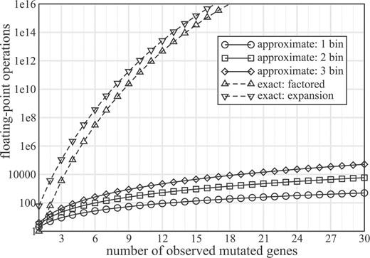
Floating-point operations as a function of the number of observed mutations for a test set of m = 60 genes for exact (dashed curves) and approximate (solid curves) solutions. Given Equation (5), all curves are symmetric about m / 2, so the plot only shows data up to k = 30.
3.2 Approximation accuracy
The approximation method in Theorem 3 gathers genes into bins and uses the average bin length as a proxy for the individual lengths. The degree of error in this process depends upon the loss of resolution of the individual gene Bernoulli probabilities. For instance, the hypothetical multiset of gene lengths {3000, 8500, 8500, 3000} can be partitioned into {3000, 3000} and {8500, 8500} without loss of resolution, i.e. it is exact. However, test sets will generally not contain such a fortuitous list of gene lengths, prompting the question of how to best partition a list of lengths. Optimal clustering in any given instance will produce j subsets, not necessarily with equivalent numbers of elements, but with each subset having minimal size variation among its elements. The general problem for m elements is not trivial (Xu and Wunsch, 2005).
Let us first sort the original lengths L1, L2, …, Lm into an ordered list L(1)≤ L(2)≤ … ≤ L(m). Optimization then requires determining how many bins should be created and where the boundaries between bins should be placed. While coding lengths of human genes vary from hundreds of nucleotides up to order 104 nt, the background mutation rate is generally not larger than order 10 − 6/nt. These observations suggest that the accuracy of using approximation (Theorem 3) would not be a strong function of partitioning because variations in the Bernoulli probabilities would not vary wildly. In other words, suboptimal partitions should not cause unacceptably large errors in calculated P-values.
We tested this hypothesis in a ‘naïve partitioning’ experiment, where the number of bins is picked a priori and then the ordered lengths are divided as equally as possible among these bins. For example, for j = 2 one bin would contain all lengths up to L(m / 2), with the remaining lengths going to the other bin. Figure 2 shows results for representative small and large gene sets using 1 bin and 3 bin approximations. Plots are made for plausible background rate bounds of 1 and 3 mutations per Mb. P-values are overpredicted, with errors being sensitive to both the number of bins and the mutation rate. From a hypothesis testing perspective, error is most critical in the neighborhood of α. Yet, we generally will not have the luxury of knowing its magnitude here a priori, or by extension, whether a gene set has been misclassified according to our choice of α. Evidently, error is readily controlled by small increases in j without incurring significantly increased computational cost. This behavior will be especially important in two regards: for controlling the error contribution of any ‘outlier’ genes having unusually long or short lengths, and for the ‘matrix problem’ of testing many hypotheses using many genomes, where substantially lower adjusted values of α will be required (Benjamini and Hochberg, 1995). Note that Figure 2 results are simulated in the sense that the gene lengths were chosen randomly. Errors realized in practice could be less if size variance is correspondingly lower. A good general strategy may be to always use at least 3-bin approximation in conjunction with naïve partitioning.
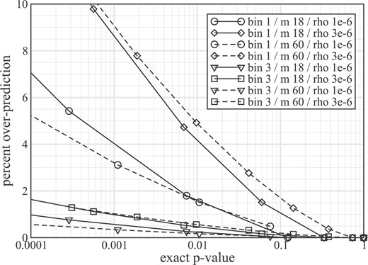
Percent overprediction of P-values from representative small (m = 18, solid curves) and large (m = 60, dashed curves) gene sets. Four scenarios are considered: j = 1 bin with background mutation rate of ρ = 1/Mb (circles), j = 1 and ρ = 3 (diamonds), j = 3 and ρ = 1 (triangles), and j = 3 and ρ = 3 (squares). Test sets were generated with randomly selected lengths between 200 and 15 000 nt.
There is necessarily a second level of approximation in combining the sample-specific P-values from many genome samples into a single, project-wide value. These errors are not readily controlled at present because the fundamental mathematical theory underlying combined discrete probabilities remains incomplete. Moreover, obtaining any reliable assessment against true population-based probability values, i.e. via exact P-values and their subsequent exact ‘brute-force’ combination, is computationally infeasible for realistic scenarios. It is important to observe that all tests leveraging data from multiple genomes will be faced with some form of this problem, though none evidently resolve, acknowledge or perhaps even recognize it. The implications are substantial, as we demonstrate below when comparing to the so-called pooled statistical methods.
3.3 Statistical power analysis
Power analysis is useful for characterizing the minimum conditions for which an effect would be reasonably detectable (Sokal and Rohlf, 1981). Recall, H0 is based on the premise of a random underlying mutation rate ρ. Mutations should be more frequent in true cancer-related sets, implying we could estimate power based on the simple alternative hypothesis, H1, of a process characterized by some elevated, cancer-specific mutation rate,  (Parmigiani et al., 2008). There is a necessary degree of speculation here, as we have no reliable information regarding such a rate. It would presumably vary by tumor stage and grade, by cancer type, by individual, etc., so a given value would not be representative of cancer in any general sense. This echoes earlier points regarding the difficulties of accurately assessing power (Tarca et al., 2009). Let us simply examine this issue on the basis of a plausible lower bound, / ρ = 2, and a perhaps conservative upper bound, / ρ = 5, respectively. Calculation methodology is detailed in Supplementary Material.
Figure 3 shows power curves at α = 1% for several sample sizes, where ρ is taken as three mutations per megabase. If differences in cancer and background rates are on the order of only 2-fold, small pathways will remain undetectable unless sample size is extremely large. For example, a 10 gene pathway nets only about 30% power for 25 sequenced genomes. Conversely, the value jumps to almost 100% for a 5-fold difference in mutation rates. Discovery of small pathways is clearly very sensitive to the true cancer mutation rate, which requires better characterization to make suitably accurate predictions. For larger gene sets, e.g. m≥ 100, extrapolation (Supplementary Material) suggests that power will be acceptable regardless of the cancer mutation rate. For example, sequencing 25 genomes is now basically feasible using next-generation instrumentation and this sample size puts power near 100%, even for fairly small differences between the cancer and background mutation rates.
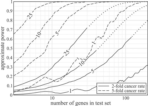
Estimated statistical power as a function of test set size for α = 1%. Solid and dashed curves represent assumed cancer mutation rates of 2-fold and 5-fold higher than the background rate (ρ = 3/Mb), respectively. Dotted curves denote extrapolation beyond computational limits of the 2-fold results based on least–squares fitting (Supplemental Information). All calculations were made using the 3-bin approximate solution on randomly generated test sets having gene lengths between 200 bp and 15 kb. Each datum indicates the average of 100 such trials.
3.4 Comparison to other tests
PathScan is admittedly not the first pathway test to be developed or applied for cancer analysis. So-called ‘pooled techniques’ have already been used for quite some time. These procedures simply combine total mutations and total mutable positions in a gene set into single respective tallies, calculating significance directly from, for example, Fisher's test (mutation rate within pathway versus rate outside of pathway) or binomial or Poisson distributions (observed mutation count in the light of an estimated background rate). The Group-CaMP test (Table 1) is perhaps the most well-known of these tally methods (Lin et al., 2007). This elementary class of tests harbors a critical liability in the form of significant information loss that necessarily follows from discarding both the distribution of gene lengths in γ and the distribution of mutations among samples. While the implications of the former are readily understood in terms of differing gene mutation probabilities (Theorem 1), the latter aspect is less apparent. Consider the following.
The essential problem is that simple tallies cannot distinguish between a few genes having multiple mutations versus many genes having only a few mutations apiece in a group of samples (Fig. 4). Let us borrow a common, but elementary example from the statistics literature (Lancaster, 1949; Wallis, 1942) to illustrate this point, i.e. (n, m, b) = (2, 4, 0.5). Here, each gene has an equal mutation probability. Binomial pooling reduces this problem to a simple tallying scenario having a maximum n ċ m = 8 potential mutations, where probability masses are  . For example, for k = 6, calculations return PK ≥ 6≈ 0.145. However, pooling is not actually able to distinguish differences in how mutations could be distributed among the samples. There are two possibilities here for k = 6: four mutations in one sample and two in the other or three in each sample (Fig. 4), with the latter being about a third more probable.
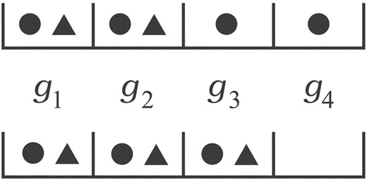
Two mutation scenarios for (n, m, b, k) = (2, 4, 0.5, 6). The top panel represents a 4 + 2 configuration, i.e. all 4 genes mutated in one sample (circles) and only two genes mutated in the other sample (triangles), while the bottom panel is a 3 + 3 configuration. Pooled statistics are unable to distinguish between these two scenarios, even though their significance values are appreciably different, i.e. ≈ 0.047 for the top panel and ≈ 0.063 for the bottom (Wallis, 1942).
This example has been solved exactly via enumeration (Wallis, 1942), from which we find the true P-value PK ≥ 6≈ 0.184. The explanation for the perhaps surprising difference is that there are actually several configurations having fewer than six mutations, which are nevertheless more significant than the 3 + 3 configuration. These cases, 0 + 4 and 1 + 4, are necessarily omitted from the pooling calculation because of its loss of resolution. Combinatorial considerations indicate that such ‘out-of-rank’ mutation probabilities multiply enormously as the numbers of genes and samples increase, implying increasingly large errors in the resulting P-values. Our opinion in the light of this observation is that simple statistical pooling methods are no longer tenable.
3.5 Example calculation
We applied PathScan to the Tumor Sequencing Project (TSP) lung adenocarcinoma gene set data in order to extend the calculations originally performed by (Ding et al., 2008) to find significantly mutated KEGG pathways (Kanehisa et al., 2010). The TSP study used two tally-based tests: a binomial model based on a background rate of three mutations per megabase and a Fisher exact test of gene mutations within the subject pathway versus those outside the pathway. Our results are compared to these computations in Supplementary Table S1. The following cases have been redacted from this table: (i) known cancer pathways whose mutation lists are invariably dominated by a few known cancer genes, especially TP53, KRAS and EGFR, (ii) other pathways whose mutations likewise reside in just a single gene, (iii) pathways having only a single mutation, and (iv) pathways not appearing in the original TSP study. In all, 129 pathways were examined and we based our multiple-testing correction (Benjamini and Hochberg, 1995) on this figure.
Not surprisingly, our calculations recapitulate the same pathways found to be highly significant by the two TSP tests. Their P-values differ from one another by orders of magnitude and both differ similarly from our own results, which are generally much less extreme. Yet, all these differences are vastly outweighed by the extent to which each P-value surpasses a standard 1% threshold. Significant members include the signaling pathways MAPK and mTOR.
The more relevant cases for our assessment purposes are ones for which the original TSP tests were prima facie inconclusive, i.e. where the two calculations disagreed. Importantly, the extent of these disagreements is always several orders of magnitude in the P-value. In other words, the ambiguity in such cases is not simply a result of how FDR is chosen, but instead reflects the inherent problems of tally-based tests we described above. For example, the binomial TSP test counted taste transduction (hsa04742) and Alzheimers disease (hsa05010) as significant, while the Fisher TSP test did not. The converse list includes Toll-like receptor signaling (hsa04620), Jak-STAT signaling (hsa04630), and leukocyte transendothelial migration (hsa04670). PathScan concludes that none of these pathways is significant.
On the other hand, PathScan finds several of the previously inconclusive pathways to actually be significant, the biologically most interesting example being focal adhesion (hsa04510). Focal adhesions are large protein complexes linking the cell cytoskeleton with the extracellular matrix. They transmit regulatory signals affecting many cellular processes including motility, proliferation, differentiation, regulation of gene expression and cell survival. These functions immediately imply various possible physical relevancies to cancer. Moreover, this pathway has been found to be significantly affected in gene expression studies on prostate cancer (Huang and Chow, 2007), ovarian cancer (Crijns et al., 2009) and proliferative breast lesions (Emery et al., 2009).
We went a step further, expanding calculations for the mutated TSP gene list to six databases: BioCarta (Nishimura, 2001), KEGG (Kanehisa et al., 2010), PID (Schaefer et al., 2009), Pfam (Bateman et al., 2000), Reactome (Joshi-Tope et al., 2005) and SMART (Letunic et al., 2009). These resources collectively furnish 988 tests of individual gene groupings and we use this figure for our FDR correction. Table 2 shows 25 candidates that remain after a redaction process similar to that described above. In other words, these groupings all have both a significant FDR and a mutation list containing a good variety of gene hits. In addition to the KEGG focal adhesion pathway, there are several other notable hits that we highlight here.
Significant lung adenocarcinoma groupings from six databases
| # | Database | Pathway description | FDR |
|---|---|---|---|
| 1 | KEGG | hsa04010: MAPK signaling | 3.0e-42 |
| 2 | Pfam | PF07714: Pkinase Tyr | 5.9e-26 |
| 3 | SMART | SM00219: TyrKc | 2.0e-25 |
| 4 | Reactome | REACT 18266: axon guidance | 1.8e-18 |
| 5 | KEGG | hsa04012: ErbB signaling | 6.5e-18 |
| 6 | KEGG | hsa04020: calcium signaling | 1.0e-12 |
| 7 | Pfam | PF07679: I-set | 3.8e-12 |
| 8 | Reactome | REACT 11061: signalling by NGF | 1.1e-11 |
| 9 | KEGG | hsa04144: endocytosis | 3.2e-10 |
| 10 | SMART | SM00408: IGc2 | 3.0e-09 |
| 11 | PID | regulation of telomerase | 3.5e-09 |
| 12 | KEGG | hsa04060: cytokine interaction | 5.4e-09 |
| 13 | KEGG | hsa04510: focal adhesion | 1.8e-08 |
| 14 | SMART | SM00060: FN3 | 7.8e-07 |
| 15 | Pfam | PF00041: fn3 | 7.8e-07 |
| 16 | BioCarta | h_her2Pathway | 8.7e-07 |
| 17 | PID | signaling events mediated by PTP1B | 1.7e-06 |
| 18 | PID | Thromboxane A2 receptor signaling | 3.3e-06 |
| 19 | KEGG | hsa04520: adherens junction | 2.0e-05 |
| 20 | PID | endothelins | 2.9e-05 |
| 21 | SMART | SM00409: IG | 1.9e-04 |
| 22 | KEGG | hsa04150: mTOR signaling | 3.6e-04 |
| 23 | SMART | SM00220: S_TKc | 2.8e-03 |
| 24 | PID | EPHA forward signaling | 0.008 |
| 25 | BioCarta | h_no1Pathway | 0.0094 |
The ErbB signaling pathway (Table 2, hit 5) is activated by extracellular growth factor binding to one of four structurally related receptor tyrosine kinases, EGFR, ERBB2, ERBB3 or ERBB4. Excessive ErbB signaling has been implicated in the development of a wide variety of solid tumors (Hynes and MacDonald, 2009). The large number of mutations in ERBB4, EGFR as well as in downstream genes such as KRAS, PAK3 and PIK3CG contribute to the highly significant P-value calculated by PathScan for this pathway. Replicative senescence, growth arrest caused by progressive shortening of telomeres during cell division, is thought to be bypassed in most tumors (Shay and Wright, 2002). The telomerase regulation pathway (hit 11) is significantly affected in the samples surveyed, showing mutations in pathway genes such as EGFR, ATM, TERT and others. Notably, TERT has been found to be significantly amplified in lung adenocarcinoma (Ding et al., 2008). The EPHA pathway (hit 24) plays various roles in vertebrate and invertebrate development by regulating cell position and morphology. Disregulated EPHA signaling has been associated with cancers from breast, colon, prostate and esophagus and the Eph receptors are a promising drug target (Pasquale, 2010). In addition to mutations in the receptors EPHA1 through EPHA7, mutations in pathway genes such as FYN and HCK were identified in lung adenocarcinoma.
4 CONCLUSION
The statistical testing spectrum for cancer DNA sequence is growing rapidly. We have proposed a new method that considers the variable Bernoulli probabilities for differing gene sizes under the null hypothesis and systematically treats the combination of sample-specific P-values in order to obtain a population-based value for a large set of samples. In short, this procedure retains several important pieces of information that existing models discard. Moreover, the method accounts for these factors in a way that does not add significant computational liabilities by using the mathematical concepts of convolution and Fisher–Lancaster theory.
The model is easily extended to more general scenarios. For example, growing bodies of data will allow increasingly accurate assignments of gene-specific background mutation rates, ρi. Yet, because we already assume gene-specific Bernoulli values, it is trivial to generalize Theorem 1 as bi = exp (− ρiLi) without incurring any net increase in CPU cost. This property will also permit integration of other phenomena, including copy number changes, structural variation and methylation and expression changes, should it become possible in the future to assign meaningful Bernoulli values to such events. This last aspect is especially relevant. The cancers are a complex family of diseases and it will be important to broaden investigations to integrate all the types of aberrations that could be linked to a specific phenotype.
The integration problem is actually just one part of a broader research program of pathway analysis. For example, there remains no conclusive method to differentiate the action of a gene from that of a pathway in those cases where the mutation list is dominated by one gene. Although we have shown that PathScan suffers vastly less from this phenomenon than other tests, it does not fully solve this problem. Development of supplemental ‘exclusionary’ tests that specifically examine distributions of mutations among member genes may be necessary. Moreover, models do not yet systematically account for relationships or conditioning that may exist between specific mutations in a network sense, i.e. considering the position and role of a mutated gene within its pathway, multiple gene functions, etc.
PathScan is applicable to any set of genes, γ, no matter how constructed, meaning it is useful both with pathway databases, as we have shown here, and in de novo network-building methods that use interaction databases. The latter must ultimately evaluate network significance in the context of the associated somatic events and often still resort to elementary tests (Glaab et al., 2010). Irrespective of method, any calculation is necessarily limited by whatever databases it uses (Cerami et al., 2010; Vandin et al., 2010). However, because the collective wealth of stored information continues to increase at a remarkable rate (Kanehisa et al., 2010), such concerns should diminish over time.
These observations all suggest that future methods will necessarily become more sophisticated and increasingly focused on the deeper aspects of cancer genomic analysis. We feel that PathScan represents an initial, though deliberate step in that direction.
ACKNOWLEDGEMENTS
The authors appreciate Michael McLellan's assistance with analysis files and bioinformatics support.
Funding: Grant (HG003079) from the National Human Genome Research Institute (to R.K.W., PI).
Conflict of Interest: none declared.
REFERENCES
Author notes
Associate Editor: Alfonso Valencia

