


Abstract
Motivation: Chromosomal aberrations tend to be characteristic for given (sub)types of cancer. Such aberrations can be detected with array comparative genomic hybridization (aCGH). Clustering aCGH tumor profiles aids in identifying chromosomal regions of interest and provides useful diagnostic information on the cancer type. An important issue here is to what extent individual aCGH tumor profiles can be reliably assigned to clusters associated with a given cancer type.
Results: We introduce a novel evolutionary fuzzy clustering (EFC) algorithm, which is able to deal with overlapping clusterings. Our method assesses these overlaps by using cluster membership degrees, which we use here as a confidence measure for individual samples to be assigned to a given tumor type. We first demonstrate the usefulness of our method using a synthetic aCGH dataset and subsequently show that EFC outperforms existing methods on four real datasets of aCGH tumor profiles involving four different cancer types. We also show that in general best performance is obtained using 1− Pearson correlation coefficient as a distance measure and that extra preprocessing steps, such as segmentation and calling, lead to decreased clustering performance.
Availability: The source code of the program is available from http://ibi.vu.nl/programs/efcwww
Contact: [email protected]
Supplementary information: Supplementary data are available at Bioinformatics online.
1 INTRODUCTION
Array comparative genomic hybridization (aCGH) is an experimental approach that allows researchers to scan entire genomes for copy number changes at high resolution. These changes occur due to mutation, resulting in either gain or loss of genetic material. Chromosomal copy number changes are common features of malignant tumor cell lines. Interestingly, different types of cancer appear to have different numerical and structural chromosomal imbalances (Jong et al., 2007; Meza-Zepada et al., 2006). The same might be true for subtypes of cancer (Jonsson et al., 2005; Pollack et al., 2002). Moreover, a correlation has been observed between copy number changes and clinical observations such as patient survival or responsiveness to certain treatments (Van Wieringen et al., 2008; Weiss et al., 2003). This means that detecting copy number changes can not only identify chromosomal regions of interest but also provides useful diagnostic information on the cancer type. Accurate diagnosis in turn, allows for more accurate prognosis and targeted treatment.
To distinguish different (sub)types of cancer based on copy number changes, clustering algorithms are often used. Different algorithms and techniques for clustering exist, but to date basic hierarchical clustering is commonly used for aCGH data analysis (e.g. Fridlyand et al., 2006; Jong et al., 2007; Jonsson et al., 2005). Liu et al. (2006) propose three measures to quantify the distance between two CGH samples and evaluate them using hierarchical clustering and k-means. They obtain best performance using agglomerative hierarchical clustering in combination with one of their measures named Sim, which measures the number of independent common aberrations. Van Wieringen et al. (2008) were the first to propose a clustering method tailored to called aCGH data. They introduce two novel distance measures (one of which is a generalization of Sim) and a novel hierarchical clustering criterion. Their method, called weighted clustering of called aCGH data (WECCA), also allows for weighting the clones (or regions), but is computationally intensive.
The popularity of hierarchical clustering is based on the fact that it generates a dendrogram, which allows researchers to get a quick notion of the underlying structure of the data. The approach suffers from some major problems, however. It has been noted to suffer from the lack of robustness and non-uniqueness (Morgan and Ray, 1995). Furthermore, the greediness of hierarchical clustering can cause objects to be grouped based on local decisions, with no opportunity to re-evaluate the clustering. Also, hierarchical clustering cannot represent distinct clusters, except by ‘cutting’ the dendrogram at a certain (arbitrary) point. Furthermore, strict phylogenetic trees are best suited to situations of true hierarchical descent such as in the evolution of species (Tamayo et al., 1999), which is not necessarily the case for aCGH data.
Another popular technique is k-means clustering (MacQueen, 1967) as it is fast, easy to interpret, easy to implement and always converges to local optima. On the other hand, k-means is easily trapped in local optima (Hartigan, 1975) and not robust to noise and outliers. For example, addition of a single sample to a cluster can radically change the outcome of the algorithm (Bezdek, 1998).
Hierarchical and k-means clustering force each aCGH profile into exactly one cluster, which is called hard clustering. This disregards the fact that different tumor types often have aberrations in common. For example, the genes PIK3CA (a tumor suppressor gene on human chromosome 3) and TP53 (a p110α protein-encoding gene on human chromosome 17) co-occur frequently in both breast and colorectal cancers (Wood et al., 2007). This means that aCGH tumor profiles or parts thereof could correspond to more than one group. Fuzzy clustering algorithms, such as Fanny (Kaufman and Rousseeuw, 1990), fuzzy k-means (Bezdek, 1973; Dunn, 1973) and fuzzy j-means (Belacel et al., 2002) take possible overlap of aberrations into account by using membership degrees, which express the relative likelihood of each object to pertain to each of the clusters. Membership degrees have the advantage that they not only can be interpreted as a degree of belongingness, but also as a degree of confidence for the objects to belong to a given cluster. This information is not available if hard clustering is performed.
In this article, we consider a new approach for clustering aCGH data. Our aim is to construct a clustering algorithm for analyzing aCGH profiles, which (i) is able to deal with overlapping clusters; (ii) identifies and downweights outliers on the fly; and (iii) has a high chance of finding the ‘true’ clustering. To achieve this, we use fuzzy clustering as a starting point. This technique involves minimizing an objective function by appointing optimal membership degrees of aCGH profiles to cluster centroids. We use an evolutionary algorithm to perform the optimization, which are known to be relatively insensitive to local optima.
We also present two novel genetic operators in our evolutionary algorithm, specially designed to guide and speed up the evolutionary clustering process. The first new operator is 1-step k-means, a mutation operator inspired by the k-means algorithm. Next, sorted 1-point crossover is derived from simple 1-point crossover. Sorting the cluster centroids in advance is expected to prevent the recombination for being too disruptive.
2 METHODS
2.1 Objective function
2.2 The optimization algorithm
The task at hand now is to minimize the objective function (3), in order to obtain the optimal clustering. We have chosen to use a Genetic Algorithm (GA; Holland, 1975) to perform this minimization.
2.2.1 Representation of the GA individual
Representation and exploration of the problem parameter space can be based on encoding and evolving either of the variables U and V, where one variable can be eliminated and optimization of the objective function (3) is performed over the other. Presenting the parameter space with U has the disadvantage that the GA chromosome is proportional to the dataset size. As a consequence, operating on those GA chromosomes may require heavy calculations. We have chosen a floating point encoding of the cluster centroids as parameter space representation for our algorithm. So a GA chromosome is a c × p matrix where each row represents a cluster centroid. The parameter p denotes the dimensionality of the objects [in our case, the number of clones or regions, depending on the data version (Section 3.1)]. Given a centroid V, the membership values uij are eliminated via substitution from (2) into (3). The fitness can then be calculated from the objective function (3). This approach is permitted, as for fixed V, minimization of (3) over U can be done by applying (2) (Bezdek, 1981).
2.2.2 Recombination
We introduce a new recombination operator, called sorted 1-point crossover which recombines two parent GA chromosomes creating two offspring GA chromosomes. To prevent the recombination process for being too disruptive, the centroids of both parent GA chromosomes are first sorted by their modulus (i.e. distance to the origin). This operation does not alter the GA chromosome's phenotype, as the order of centroids within a clustering is meaningless. After sorting, a number t between [1,…, c] is randomly selected and two new child GA chromosomes are created by combining the [1,…, t] and [t+1,…, c] parts of the two parents.
2.2.3 Mutation
Several mutation operators for real coding have appeared in the literature (Herrera et al., 1998; Michalevitz, 1992). To guide and speed up the space search, and to increase the search precision, we introduce a novel heuristic for mutation, which we coin 1-step k-means. A GA chromosome is mutated by applying one cycle of the k-means algorithm using all the aCGH samples and using the GA chromosome as initialization centroids for the k-means. First, each sample is assigned to the nearest centroid. Then each centroid is recalculated as the average of all samples assigned to that centroid. In this way, the centroids make an informed move to the closest data points. Note that in the case of multiple centroids within one GA chromosome are nearby in the search space, it is possible that they become identical after the 1-step k-means mutation. As such GA chromosomes with duplicate centroids in effect comprise less clusters than required, they are removed.

2.2.4 Fitness function
As the fitness function for our GA, we take the negation of the objective function, since our objective function is to be minimized instead of maximized.
2.2.5 Selection
We use elitist (μ + λ) selection, where the best μ GA chromosomes from a set of λ offspring and μ parents are selected, while λ and μ represent the population and mating pool size, respectively. (μ + λ) selection has the advantage that convergence is guaranteed, i.e. if the global optimum is discovered, the GA converges to that maximum (De Jong, 1975). In our algorithm, we chose μ = 15 and λ = 100, which are commonly used values.
2.2.6 Algorithm
Here, the pseudo code of our algorithm is presented.

The population is initialized by creating individuals with c cluster centroids, which are initialized by assigning a randomly selected data point to them. This initialization procedure provides a good starting point for the reproduction cycle, as each cluster centroid lies close to at least one of the data points.
The algorithm is terminated as soon as the population is converged. We check this by comparing the highest and the lowest fitness values within the population. If they are (nearly) equal, the algorithm terminates. To prevent the algorithm from running too long, the algorithm is also terminated after a maximum number of generations (set to 100).
3 SYNTHETIC DATASET
To test our evolutionary fuzzy clustering (EFC) algorithm and to show the usefulness of membership degrees and weight factors, we applied it to a synthetic aCGH dataset, where we defined individuals of various points in between clusters.
3.1 Data generation and preprocessing
Each template profile contains eight ‘aberrant segments’ of 100 equally spaced clones of DNA copy number 1 (loss), 2 (normal) or 3 (gain), or of 5 clones of copy number 20 (amplification). To reflect that each sample is a mixture of tumor cells and normal cells, we chose −0.3, 0, 0.3 and 3.0 for the respective log2 ratios. The aberrant segments are interleaved with normal segments of 200 clones, or 295 clones in case of amplifications. To demonstrate the effect of overlapping clusters on the membership degrees, we constructed templates AB1 and AB2 such that they lie in the overlapping area between templates A and B. Templates AB1 and AB2 only differ in their degree of overlap with template B, which is larger for AB2. Template C2 is, apart from the amplification, identical to template C1 to assess whether clustering methods are able to pick up amplifications. A small set of outliers was generated from the Outliers template to establish their effect on the weight factors.
Synthetic data was generated by adding Gaussian noise with a standard deviation (SD) of 0.2, 0.15, 0.25 and 0.3 over the losses, normals, gains and amplifications, respectively. These values were derived from analysis of real aCGH data involving four cancer types (Section 4). This analysis comprised normalization, segmentation and calling of the data. Then, based on these calls, the normalized data were grouped into four populations: losses, normals, gains and amplifications. For each of these populations, the mean and SD were determined. We generated 25 samples from templates A, B, C1, C2 and D, whereas from the AB and Outliers templates only 10 and 5 samples were generated, respectively.
For the preprocessing of the data, we employed the R-package CGHcall (Van de Wiel et al., 2007) using median normalization (Khojasteh et al., 2005), segmentation with smoothing for outliers (Venkatraman and Olshen, 2007), and calling with four levels. As a last step, we used the CGHregions algorithm (Van de Wiel and Van Wieringen, 2007) to compress neighboring clones which are constant across samples into clone regions. Using this scenario, we created four versions of the dataset, which we will, respectively, refer to as: normalized, segmented, called clones and called regions. This allows us to additionally investigate whether preprocessing effects the clustering accuracies, and if so, in what way. All these versions of the synthetic data are available in the Supplementary Materials.
In the remainder of this article, we will refer to the set of profiles generated from template X as profile class X.
3.2 Results
We compared the performance of EFC with the clustering methods k-means, complete linkage, Ward's linkage and WECCA's total linkage (Van Wieringen et al., 2008). The comparison was made for all four preprocessed versions of the dataset in combination with five different similarity/distance measures, namely Euclidean distance, Pearson correlation, Spearman rank correlation and WECCA's agreement and concordance. It should be noted that total linkage is only defined in combination with agreement and concordance and that these similarity measures are, in turn, only defined for called data, hence runs for other similarity/distance measures or preprocessed data were not feasible. Furthermore, as EFC and k-means are non-deterministic such that subtle differences in results may occur, we run these algorithms 100 times on each of the settings.
The data were clustered into five groups, since profile class A, B, C1, C2 and D should form one cluster each. Samples from profile class AB1 and AB2 should be clustered together with those of A or B. The profile class Outliers must be assigned a weight factor below 0.75 in order to be disregarded in the results.
Results on the performances of each clustering method are shown in Table 1. The best overall accuracy of 100% is achieved by EFC, as well as by complete and Ward's linkage. All three methods show this performance on both normalized and segmented data for at least one distance measure. Complete and Ward's linkage also yield a perfect clustering on called regions data, whereas EFC performs nearly perfect there with accuracies of 96.5, 98.8 and 96.8% (using Euclidean, Pearson, and agreement distance, respectively). With respect to the called clones data, Ward's linkage shows best performance with an accuracy of 82.8% using the Pearson and Spearman distance. Also here, EFC is only a fraction behind with accuracies of 82.6 and 82.5% using the Pearson and concordance distance, respectively. It is striking that on called data (both clones and regions), WECCA's total linkage is outperformed by EFC, complete linkage and Ward's linkage, although total linkage has been specifically designed for this type of data. Regarding the distance measures, it is clear that in general best results are achieved with the Euclidean or Pearson distance.
Performance of clustering algorithms compared with respect to the synthetic aCGH dataset after different preprocessing steps, using different distance measures
| Distance measure | EFC | k-means | Complete | Ward's | Total | |
|---|---|---|---|---|---|---|
| linkage | linkage | linkage | ||||
| Normalized | Euclidean | 90.5 (8.05) | 93.7 (8.90) | 100 | 100 | |
| 1−Pearson | 100 (0.00) | 90.4 (9.77) | 79.2 | 100 | ||
| 1−Spearman | 59.1 (9.00) | 49.9 (1.35) | 79.2 | 75.9 | ||
| Segmented | Euclidean | 100 (0.00) | 82.7 (2.97) | 100 | 100 | |
| 1−Pearson | 100 (0.00) | 76.6 (18.3) | 79.2 | 100 | ||
| 1−Spearman | 59.0 (6.51) | 48.7 (6.33) | 53.8 | 59.3 | ||
| Called clones | Euclidean | 75.9 (0.00) | 68.3 (4.59) | 79.2 | 75.9 | |
| 1−Pearson | 82.6 (1.18) | 62.1 (6.90) | 79.2 | 82.8 | ||
| 1−Spearman | 79.4 (3.45) | 76.4 (8.78) | 79.2 | 82.8 | ||
| 1−Agreement | 76.8 (4.06) | 17.2 (0.07) | 58.6 | 75.9 | 58.6 | |
| 1−Concordance | 82.5 (7.24) | 60.7 (7.74) | 58.6 | 75.9 | 58.6 | |
| Called regions | Euclidean | 96.5 (0.00) | 74.6 (7.55) | 100 | 96.6 | |
| 1−Pearson | 98.8 (2.94) | 82.6 (0.82) | 83.4 | 96.6 | ||
| 1−Spearman | 98.8 (2.02) | 43.9 (13.5) | 79.2 | 100 | ||
| 1−Agreement | 96.8 (3.60) | 30.0 (15.3) | 100 | 96.6 | 83.4 | |
| 1−Concordance | 77.7 (12.0) | 65.9 (13.7) | 82.8 | 100 | 82.8 |
Numbers are accuracies (averaged over 100 runs, in case of EFC and k-means), numbers between brackets are SDs, numbers in boldface represent the best accuracy per preprocessing stage (normalized, segmented, called clones and called regions).
Next we assessed the added value of our two novel GA operators 1-step k-means and sorted 1-point crossover. To this end, we performed a full rerun of EFC in three different modes: (i) simple random mutation instead of 1-step k-means, (ii) no sorting before 1-point crossover and (iii) both adjustments. For each version, the overall average performance over all runs was recorded. The results of this comparison are presented in Table 2. The version including the two novel GA operators shows the highest average performance with an accuracy of 88.0%, against 81.8% for the version without the novel operators. 1-step k-means appears to have the highest contribution in the increase of the performance, since an accuracy of 87.7% is reached including this operator. Sorting before the 1-point crossover adds at most a few percentage points to the performance.
Assessment of the two novel GA operators 1-step k-means and sorted 1-point crossover
| 1-Point crossover | ||
|---|---|---|
| Non-sorted | Sorted | |
| Random mutation | 81.8 (15.3) | 83.5 (15.3) |
| 1-step k-means | 87.7 (14.6) | 88.0 (14.6) |
| 1-Point crossover | ||
|---|---|---|
| Non-sorted | Sorted | |
| Random mutation | 81.8 (15.3) | 83.5 (15.3) |
| 1-step k-means | 87.7 (14.6) | 88.0 (14.6) |
Different versions of EFC with and without these operators were compared on the synthetic aCGH dataset. Numbers are accuracies averaged over all combinations of preprocessing stages (normalized, segmented, called clones and called regions) and distance measures (Euclidean distance, Pearson correlation, Spearman rank correlation, agreement and concordance). Numbers between brackets are SDs.
We also recorded the resulting membership degrees and the weight factors for the EFC runs on the generated data using 1−Pearson correlation as a distance measure. Figure 1 shows the resulting membership degree distribution over the fuzzy clusters. Profile classes A, B and D, which are designed not to be overlapping, clearly show a high average membership degree (u > 0.8) to their corresponding clusters, indicating that there is no overlap indeed. Profile class AB1, on the other hand, was designed to share many characteristics with profile class A and some with B, which EFC properly translates into membership degrees to the corresponding clusters of 0.74 and 0.18, respectively. The membership degrees of profile class AB2 are reasonably equally divided over clusters A and B (u = 0.45 and u = 0.49, respectively), adequately reflecting that AB2 was designed to be equally similar to profile classes A and B.
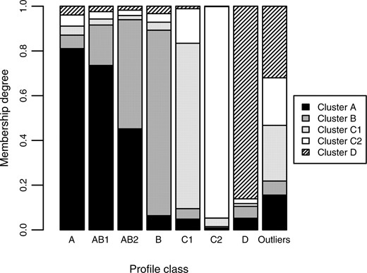
Barplot illustrating that membership degrees adequately capture overlapping clusters. Results are averages of all synthetic samples per profile class over 100 different EFC runs. As expected, profile classes A, B and D show a high membership degree (>0.8) to their corresponding cluster, while the profile classes AB1 and AB2 show high membership degrees to both cluster A and B. Also, the intrinsically higher overlap of template profile AB2 (in comparison to AB1) with template profile B is clearly translated into a higher membership degree to cluster B.
The last step is to verify if ECF assigns a proper weight factor ωj to each artificial aCGH profile j. Remember that we set the constraint ∑j=1n ωj = n, so  . In this setting, outliers should be assigned weight factors significantly below
  . The results in Figure 2 show that EFC indeed correctly distinguishes outliers from the regular aCGH profiles. The median weight factor of the class Outliers is 0.63, which is clearly lower than 1, whereas the non-outlier profile classes are assigned weight factors close to 1 (medians range from 0.9 to 1.5). Note that samples from profile class C2 are assigned relatively the weight factors (median ωC2 = 1.5). The rationale here is that these aCGH profiles fit exceptionally well to the data, as they are similar to profiles from both the classes C1 and C2.
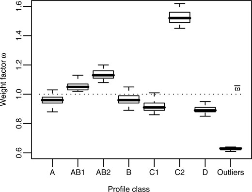
Boxplot showing that weight factors adequately capture outliers. Results are the aggregate of 100 different EFC runs. The dotted line represents the mean weight factor  , which equals 1. Samples located far below this line are considered outliers. From the graph it becomes clear that samples from the class Outliers (that were designed as outliers) are indeed assigned low weight factors (median ωOutliers = 0.63). Samples from profile class C2, on the other hand, are assigned relatively high weight factors, as they fit well in both clusters C1 and C2.
4 TUMOR DATASETS
We also applied our EFC algorithm to a set of tumor data, which is compiled from four published aCGH datasets involving four different cancer types.
4.1 Data description and preprocessing
The tumor dataset consists of the results from 102 microarray experiments of frozen tissue samples from four different cancer types, namely colorectal (20 samples), gastric (17 samples), lymphoma (41 samples) and head and neck (24 samples). All experiments have been performed in the same lab using identical BAC clones (3500–4000) as targets on the microarrays. The head and neck data were published in Smeets et al. (2006), while the other datasets were published in Jong et al. (2007).
We preprocessed each dataset in a similar fashion as the synthetic data (Section 3.1). Afterwards, we merged the different datasets on clone name (target), leaving us with 2580 BAC clones that had valid values in all samples. Also here, we end up with four versions of the data: normalized, segmented, called clones and called regions. All these versions of the tumor data are available in the Supplementary Materials, as well as the related profile plots.
4.2 Results
We compared the performance of EFC with the clustering methods k-means, (hierarchical) complete linkage and WECCA's total linkage (Van Wieringen et al., 2008) in a similar manner as with the synthetic data.
In Figure 1 of the Supplementary Materials, an EFC clustering of the tumor profiles is plotted, including the centroid for each cluster (as determined by EFC). The figure shows that, despite the large variation of the data, all clusters are adequately represented by their centroids. As expected, these centroids clearly show a distinct pattern for each tumor type. However, we also observe similarities between patterns, such as a gain of chromosome 20 in both the ‘gastric’ and ‘colon’ cluster.
Results on the performances of each clustering method are shown in Table 3. EFC clearly shows the best overall performance with an accuracy of 83.4% (±1.43) on normalized data using the Pearson correlation coefficient. Also for segmented data, called clones data and called regions data, EFC outperforms the other methods with accuracies of 71.8% (±1.18), 70.6% (±1.69) and 67.8% (±2.08), respectively. For normalized and called clones data, Ward's linkage performs similarly well. Again, as for the synthetic data, EFC outperforms WECCA's total linkage on called data. EFC is also very robust, indicated by the generally low SDs of the accuracies compared with those of k-means.
Performance of clustering algorithms compared with respect to aCGH data from four different cancer types (lymphoma, head and neck, gastric and colon; 102 samples in total) after different preprocessing steps, using different distance measures
| Distance measure | EFC | k-means | Complete | Ward's | Total | |
|---|---|---|---|---|---|---|
| linkage | linkage | linkage | ||||
| Normalized | Euclidean | 69.0 (5.06) | 67.8 (6.82) | 48.5 | 72.5 | |
| 1−Pearson | 83.4 (1.43) | 73.3 (7.62) | 77.3 | 83.3 | ||
| 1−Spearman | 78.1 (1.10) | 70.7 (8.43) | 58.5 | 79.4 | ||
| Segmented | Euclidean | 64.7 (3.26) | 64.2 (3.75) | 47.4 | 65.7 | |
| 1−Pearson | 70.1 (0.99) | 63.3 (4.92) | 66.3 | 64.7 | ||
| 1−Spearman | 71.8 (1.18) | 64.3 (7.58) | 48.4 | 68.6 | ||
| Called clones | Euclidean | 66.3 (3.55) | 66.9 (3.32) | 51.6 | 70.6 | |
| 1−Pearson | 70.6 (1.69) | 56.3 (6.36) | 50.5 | 70.6 | ||
| 1−Spearman | 65.9 (1.42) | 56.8 (6.39) | 70.5 | 70.6 | ||
| 1−Agreement | 58.9 (5.59) | 56.7 (3.04) | 48.4 | 64.2 | 60.0 | |
| 1−Concordance | 52.6 (6.07) | 61.4 (6.20) | 45.3 | 66.3 | 66.3 | |
| Called regions | Euclidean | 67.3 (3.96) | 68.2 (4.68) | 46.3 | 68.4 | |
| 1−Pearson | 67.8 (2.08) | 64.3 (2.94) | 63.2 | 65.3 | ||
| 1−Spearman | 64.8 (1.49) | 56.6 (6.95) | 64.2 | 66.3 | ||
| 1−Agreement | 55.8 (5.33) | 56.3 (3.96) | 46.3 | 66.3 | 68.4 | |
| 1−Concordance | 53.2 (6.21) | 61.2 (6.85) | 49.5 | 65.3 | 68.4 |
Numbers are accuracies (averaged over 100 runs, in case of EFC and k-means), numbers between brackets are SDs, numbers in boldface represent the best accuracy per preprocessing stage (normalized, segmented, called clones and called regions).
Comparing the results for the different preprocessing stages, best results are consistently obtained on normalized data. There are three possible explanations for this. First, information in the data may have been removed during the segmentation and calling procedure. Due to the smoothing nature and imperfection of these methods, important discriminative patterns in the data, such as heterogeneity in the DNA copy number profiles, could be lost. Secondly, some distance measures used (in particular Pearson's and Spearman correlation) are not able to handle the segmented and called data very well because of the long stretches with identical values. Thirdly, the clustering of normalized data is possibly enhanced by differences in variance levels between distinct tumor types. Since these differences in variance are removed by segmentation and calling, the clustering methods cannot make use of the variance signals. This possibly explains the decreased performances. However, for this study, we can rule out the third possibility since the differences in variances are too small [the mean variance ranges from 0.029 (lymphoma) to 0.065 (colon)] to have any significant effect on the clustering outcome.
If we compare performances of the different distance measures, we do not observe a clear winner. Overall, EFC performs best using the Pearson's correlation coefficient. The k-means method, on the other hand, generally performs best using the Euclidean distance, and complete linkage seems to work best in combination with the Spearman rank correlation. The similarity measures Agreement and Concordance only yield good performances using the WECCA total linkage method, though EFC still performs better.
As we mentioned in Section 1, membership degrees could serve two purposes: capturing overlapping clusters and ascertaining levels of confidence. To investigate possible overlaps, the membership degrees obtained by EFC are visualized as a tetrahedron in Figure 3. Here, each corner corresponds to one cluster centroid, and distances of sample points to these corners are inversely proportional to their associated membership degrees. Hence, samples having a high membership degree with respect to just one cluster will be located near the corresponding corner, whereas samples displaying characteristics of two (or more) tumor types are located in the area in between the corresponding corners. In our tumor data, we observe a clear overlap of the gastric and colon clusters involving seven samples. Also, numerous lymphoma samples show a (relative) high membership degree toward the gastric and/or colon clusters, whereas the head and neck samples show the clearest separation.
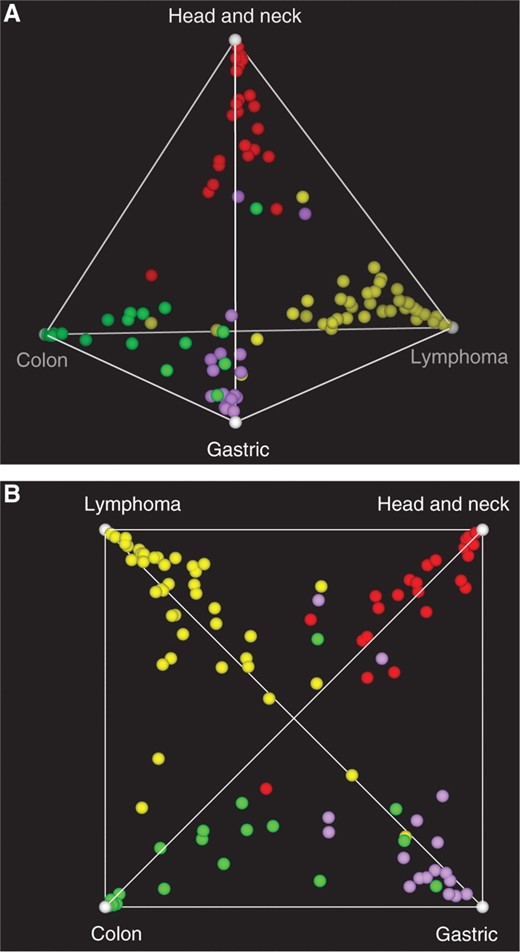
EFC reveals overlapping clusters of aCGH tumor profiles. Membership degrees are visualized as a tetrahedron, where distances of the samples to the corners are inversely proportional to the corresponding membership degrees. Lymphoma, yellow; head and neck, red; gastric, lilac; and colon, green. (A) Side view. (B) Top view. An overlap can be discerned between the colon and gastric clusters in which seven samples are involved. Furthermore, numerous lymphoma samples show a (relative) high membership degree toward the colon and/or gastric clusters, while the head and neck samples are well separated.
The weight factors ω range from 0.75 to 2.0, which means that none of these samples should be regarded as an outlier. The only exception is sample gastric_08, as it is assigned a weight factor of around 0.5 (depending on the distance measure and preprocessing stage of the data). Indeed, this is the only sample that consistently becomes grouped with clusters of a different type, and it is therefore advantageous that this sample, due to its low weight, has a reduced influence on the global clustering.
Finally, we compared the performance of the clustering methods at different noise levels. This is an important issue since high-density chips (e.g. Nimblegen, Agilent, Affymetrix) are now widely used for DNA copy number profiling albeit they suffer from very low signal-to-noise ratios. To this end, we added noise with a SD of 0.1 and 0.2 to the normalized cancer data. These data were clustered using the Pearson distance, as this appears to be the most appropriate distance measure. Total linkage was not included in this comparison, since this method can handle called data only. The results are presented in Table 4. EFC clearly shows most robustness against noise, as the performance only mildly drops from 83.4% (±1.43) to 80.6% (±1.61), whereas k-means and Ward's linkage drop about 8 percentage points in performance. Complete linkage is the least robust to noise as the performance drops almost 30 percentage points after adding noise with a SD of 0.1. However, the performance recuperates moderately after adding more noise.
Performance of clustering algorithms compared at different noise levels using aCGH data from four different cancer types (lymphoma, head and neck, gastric and colon; 102 samples in total)
| Added noise (SD) | |||
|---|---|---|---|
| 0 | 0.1 | 0.2 | |
| EFC | 83.4 (1.43) | 81.0 (2.40) | 80.6 (1.61) |
| k-means | 73.3 (7.62) | 72.0 (7.76) | 62.6 (11.5) |
| Complete linkage | 77.3 | 49.0 | 59.8 |
| Ward's linkage | 83.3 | 80.4 | 75.5 |
| Added noise (SD) | |||
|---|---|---|---|
| 0 | 0.1 | 0.2 | |
| EFC | 83.4 (1.43) | 81.0 (2.40) | 80.6 (1.61) |
| k-means | 73.3 (7.62) | 72.0 (7.76) | 62.6 (11.5) |
| Complete linkage | 77.3 | 49.0 | 59.8 |
| Ward's linkage | 83.3 | 80.4 | 75.5 |
Numbers are accuracies (averaged over 100 runs, in case of EFC and k-means), numbers between brackets are SDs.
Figure 4 shows that membership degrees as generated by EFC may also be interpreted as a level of confidence. For the tumor dataset, membership degrees of ‘correctly’ clustered samples are significantly higher than of ‘wrongly’ clustered samples. The corresponding mean values are 0.54 and 0.41, respectively. In other words, membership degrees correlate with the likelihood of an object being assigned to the ‘true’ cluster.
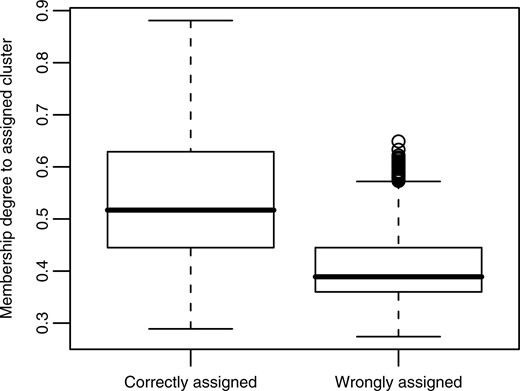
Boxplot showing that membership degrees can be used as a measure of confidence in the cluster assignment. Results are the aggregate of 100 different EFC runs. In each run, aCGH profiles from four different tumor tissues were grouped into four fuzzy clusters, which were converted into a hard clustering by assigning each aCGH profile to the cluster to which its membership degree is the highest. Then the correctness of these assignments in relation to the corresponding membership degree was assessed. The boxplot shows that, on average, correctly assigned samples have a significantly (p < 0.01) higher membership degree to their cluster than wrongly assigned ones.
5 DISCUSSION AND CONCLUSION
We introduce a novel EFC algorithm that is able to deal with overlapping clusterings and identifies outliers on the fly. Our method was tested on an artificial aCGH dataset with intrinsic overlap and outliers, and a real aCGH dataset involving four cancer types. Using the artificial dataset, we successfully demonstrate that EFC accurately groups aCGH data. Moreover, various degrees of overlap are correctly represented by intermediate membership degrees, while outliers are properly assigned significantly lower weight values. We also show the added value of the novel GA operators 1-step k-means and sorted 1-point crossover. The performance of our algorithm on synthetic and real aCGH data was compared with the conventional clustering methods k-means, complete linkage and Ward's linkage, as well as to the recently published method total linkage (Van Wieringen et al., 2008).
We conclude that for the synthetic data, Ward's linkage shows the best overall accuracy, while the performances of EFC and complete linkage are only a fraction lower. For the cancer data, EFC shows the best overall accuracy and robustness against noise, while the other methods show a lower performance. Furthermore, looking at the results on the cancer data, we observe that best performance is obtained using normalized aCGH data and 1− Pearson's correlation coefficient as distance measure. The difference in performance with the above settings compared with segmented and called data is significant. Although this tendency is less noticeable in the synthetic dataset, we think that the observed performance trends in the tumor dataset as a real biological dataset are more meaningful. Van Wieringen et al. (2007) argue that only called aCGH data should be used in downstream analyses. One of the reasons they include is the fact that normalized aCGH data are less suitable for cross-platform analyses. Another key rationale is that, in contrast to normalized and segmented data, called data have a clear biological meaning. Though this is true in principle, the actual calling to the proper biological copy number might be compromised, due to, for example, the loss of information on heterogeneity in the copy number. This is corroborated by our data (Table 3), where the four generally applicable clustering methods (EFC, k-means, complete linkage, Ward's linkage) show best performance for normalized and/or segmented data. However, we agree with (Van Wieringen et al., 2007) that more studies are needed to address this issue.
From a biological point of view, we have shown that different cancer types (colorectal, gastric, head and neck and lymphoma) can be clustered apart, solely on the basis of their copy number variations (as represented by the log2 intensity ratios). All experiments were done in the same laboratory, using the same platform, reducing the likelihood that our results are due to experimental differences. Furthermore, we have shown that head and neck cancers are more readily clustered apart, and that there is some overlap between the colorectal and gastric samples.
An added benefit of the EFC algorithm is that membership degrees can also be interpreted as a measure of confidence. We have shown that correctly assigned data points have a significantly higher membership degree on average than incorrectly assigned data points. It will be interesting to see whether these membership degrees correlate with clinical variables like survival or treatment response.
ACKNOWLEDGEMENTS
The authors would like to thank Anton Feenstra for helpful discussions and constructive comments on the manuscript. Sjoerd Vosse is acknowledged for his contribution to the data analysis, and we are grateful to Sandra Smit for her assistance in preparing the tetrahedron plot. We thank Bauke Ylstra for kindly providing the aCGH tumor datasets. Finally, we thank the anonymous referees for invaluable comments that have strengthened the article.
Funding: Bsik program ‘Ecogenomics’ (http://www.ecogenomics.nl).
Conflict of Interest: none declared.
REFERENCES
Author notes
Associate Editor: John Quackenbush

