Modified variational Bayes EM estimation of hidden Markov tree model of cell lineages Free

Abstract

1 INTRODUCTION

A central problem in stem cell biology is how a range of specialized cell types arises from a pool of stem cell progenitors. It has been reported that populations of seemingly homogeneous stem cells consist of cells which fluctuate between interchangeable sub-states (Chambers et al., 2007; Chang et al., 2008; Hayashi et al., 2008). These substates represent functionally distinct cells, which respond to stimuli in a dissimilar manner, generating diverse differentiated progeny. Heterogeneity within stem cell cultures is easily overlooked as many commonly used investigative methods rely on pooling of material before analysis. Tracking the fate of individual cells, provides a powerful method to interrogate cells in their undifferentiated state and during their differentiation. At present, the technology of tracking and monitoring cellular division and cell fate relies on the use of cells modified to carry fluorescent reporter elements to monitor changes in expression of genes known to be associated with particular cellular fates. The use of fluorescent reporter technologies is potentially limiting as it inevitably involves the alteration of the cells and realistically can only be employed to monitor up to three different parameters simultaneously. Labelling of cells using specific antibodies to cell surface proteins allows for limited monitoring of phenotype in real time, but due to the turnover of antigens in live cells requires repeated relabelling of cells with the potential perturbation of the cells characteristics. One solution to these problems is to utilize probabilistic techniques of analysis to reconstruct cell lineage trees based on observations gathered in real time (cells division rate) and combine this with particular surface antigen expression (i.e. phenotypic) information gathered at the end of the set of cell divisions being monitored.

Human embryonic stem (hES) cells spontaneously differentiate and must be constantly monitored for signs of overt differentiation. The cell surface antigen SSEA3 is rapidly down-regulated as hES cells differentiate to more mature cell types (Draper et al., 2002) and thus can serve as a useful readout of the changes in a cell's state from undifferentiated to differentiated. However, hES cells grow in tight colonies and are not amenable to real-time tracking of individual cells; therefore, the NTERA2 cell line has been used as a surrogate. The NTERA2 pluripotent cell line consists of stem cells that express the SSEA3 surface antigen at varying levels. SSEA3 expression levels have functional implications as its expression positively correlates with the probability of a NTERA2 cell to clonally expand (Andrews et al., 1984). Notably, it has been observed that NTERA2 stem cells interconvert between a SSEA3 positive and SSEA3 negative state. To determine the kinetics of this interconversion, SSEA3 negative NTERA2 cells have been obtained by fluorescent activated cell sorting and monitored by time-lapse analysis. In this study, the reconstruction of the lineage trees is based on the observations of the SSEA3 expression of the cells, where the SSEA3 expression of the cells is known only at the root and the leaf levels. There are three potential discrete states in the lineage trees: SSEA3^Positive, SSEA3^Negative or dead. The challenge consists of determining the SSEA3 expression of each cell at all levels within the lineage trees. In order to achieve this, we propose a variational Bayesian (VB) with smoothed probabilities implementation of hidden Markov trees (HMTs) which represents an analysing tool for any incomplete tree structured data. We take as our starting point the hidden Markov models (HMM), which are used in various fields such as speech recognition, financial time series prediction (Bulla and Bulla, 2006), natural language processing, ion channel kinetics (Fredkin and Rice, 1997) and general data compression (Lee, 2002). They have played important roles in the modelling and analysis of biological sequences, in particular DNA (Beerenwinkel and Drton, 2007; Schliep et al., 2005) and they have proven to be useful tools for statistical signal and image processing.

Baum and colleagues (1970) developed the core theory of HMMs. In 1972, they proposed the forward–backward algorithm as an iterative technique for the maximum likelihood (ML) statistical estimation of probabilistic functions of Markov chains. Devijver (1985) demonstrated that the computation of joint likelihoods in Baum's algorithm could be converted to the computation of posterior probabilities. The resulting algorithm was similar to Baum's except for the presence of a scaling factor suggested by Levinson et al. (1983) which was robust to computational underflow. Further developments in HMMs have come from the work of Mackay (1997), Beal and Ghahramani (2003), Watanabe et al. (2004) and Ji et al. (2006) in which they applied a VB approach to these models.

HMT models have been proposed by Crouse et al. (1997) for modelling the statistical dependencies between wavelet coefficients in signal processing. They have been applied successfully to image de-noising and segmentation (Bharadwaj and Carin, 2002; Choi and Baraniuk, 2001; Romberg et al., 2001) to signal processing and classification (Diligenti et al., 2003; Durand et al., 2004) and to tree structured data modelling (Beerenwinkel and Drton, 2007; Durand et al., 2005). The forward–backward algorithm proposed by Baum was transposed to the HMTs context by Crouse et al. (1997). The resulting algorithm has been called the upward–downward algorithm, but it suffered computational underflow problems as in Baum's algorithm. The upward–downward recursions have been proposed by Ronen et al. (1995) for the E-step in ML estimation of dependence tree models with missing observations. The upward–downward algorithm was revisited by Durand et al. (2004) who made changes to solve the computational underflow problems by adapting the ideas from Devijver's changes to the forward–backward algorithm. Romberg et al. (2001) proposed a Bayesian HMT model for image processing using wavelets and later, Dasgupta and Carin (2006) developed the VB-HMT model based on the model proposed by Crouse et al. with a similar application.

In this study, we derive the VB with smoothed probabilities implementation of HMTs. We extend Durand's HMT framework (Durand et al., 2004) to VB with the critical embodiment of prior probability distributions. Inclusion of prior probability distributions of a class of HMT models such as in the case of cell lineages is essential to avoid ill-posedness of the estimation problem. We demonstrate this through an application to modelling stem cell lineages in simulation and using real data.

2 HMT MODEL

A HMT model is composed of the observed random tree X = x₁,…, x_N and hidden random tree S = s₁,…., s_N, which has the same indexing structure as the observed tree, Figure 1. The random tree X should be viewed as containing missing observations and available observations (hence the complete tree X being of the same structure as S), for the purposes of the estimation method considered here. For example, only observations of the leaf nodes may be available and all the other x_i's can be deemed as missing observations. S takes value in a set of k discrete states, which are referred as 1,…, k. A distribution P() satisfies the HMT property if and only if:

(1)

ρ(t) represents the parent of node t, 𝒞(t) is the notation for the children of node t, X_t is the subtree rooted in t and X_1/t represents the entire tree except for the subtree rooted in t.

Fig. 1.

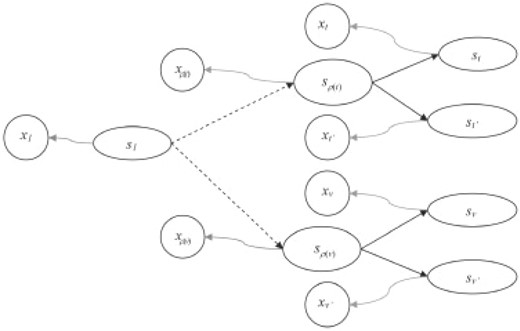
HMT representation with observed nodes (x) and hidden nodes (s). The straight arrows show the state transitions, curly arrows show emission probabilities, dashed arrows show state transitions with possibility of existence of intermediate nodes.

Open in new tabDownload slide

The parameters describing the HMT model are similar to the HMM model parameters:

for j = 1,…, k where k is the number of possible discrete values of states.

In the next sections, we will refer to all parameters of the HMT model as θ.

where vec(·) rearranges the matrix into a column vector.

3 ML ESTIMATION FOR HMT MODEL

Considering that the S states are not observable, a popular approach to determine ML estimates is the EM algorithm. For the E-step, Crouse et al. (1997) realized a direct transposition to the HMT context of the forward–backward algorithm. The result is the upward–downward algorithm which suffers from underflow problems (Ephraim and Merhav, 2002; Levinson et al., 1983). In order to overcome this, Durand et al. (2004) used an alternative decomposition of the smoothed probabilities:

(2)

The upward–downward recursions require marginal state distributions to be known. Hence, P(s₁ = j) = π_j and the recursion P(s_t = j) = ∑P_ijP(s_ρ(t) = i) have to be included in the computation.

Upward recursion for leaves of the tree:

(3)

where

Upward recursion for non-leaves:

(4)

where

and

Downward recursion based on smoothed probabilities by Durand et al. has the following expression:

(5)

At the M-step, the maximization of the expectation of log-likelihood of the complete data log 𝒬(X|θ) is realized in order to re-estimate the model parameters to be used in the next iteration.

(6)

where θ_τ+1 represents the model parameters at iteration τ + 1 and log 𝒬_τ(X|θ) is the expectation of the likelihood of the complete data with respect to the current estimate of the distribution of latent variables.

The α and β probabilities determined at the E-step are used to find the expression of log 𝒬(X|θ) as a function of parameter θ of the HMT (Ronen et al., 1995).

(7)

where the angled brackets 〈·〉 denote the expectation of a conditional probability function with respect to the missing components.

Taking the derivative of log 𝒬(X|θ) and equating to zero gives the new parameters as shown:

(8)

where λ_j,t are normalization factors which are chosen so that the probabilities sum to one,

The expression of θ mentioned above is a ML estimate, which is in the case where we do not have any prior information from the observed trees. There are circumstances where prior information is available, e.g. a node from the tree along with its parent is observed. For these cases the expression of new parameters can be written as follows:

(9)

where, as in Ronen et al. (1995), n_t^;j represents the count of the number of times that x_t = i and x_ρ(t) = j in the observed tree.

The second upwards–downward algorithm mentioned above represents the base of the E-step of the VB-EM algorithm with smoothed probabilities developed in the next section.

4 VB-EM WITH SMOOTHED PROBABILITIES ALGORITHM

The ML approach for estimating the HMT model parameters produces just a single point estimate, at the same time ML tends to overfit the data. The solutions to these problems are given by the VB approach proposed by Attias (2000). This framework applied to HMTs is able to estimate full posterior distributions over hidden variables and parameters of the model. The posterior distributions are computed via an iterative algorithm [VB-EM with smoothed probabilities (VBEMS) algorithm] that is closely related to the EM algorithm and whose convergence is guaranteed (Attias, 2000; Beal and Ghahramani, 2003). The algorithm proposed here for HMT uses the same strategy as the algorithm proposed for HMM by Mackay (1997) and Beal and Ghahramani (2003). In this study, the VB framework is adapted to HMT in similar fashion to Dasgupta and Carin (2006) but instead of using the simple upward–downward algorithm for the E-step we used the upward–downward method with smoothed probabilities. The aim is to determine the posterior probability distribution of the hidden variables S and parameters θ based on the set of observed variables X. For most model structures, the exact deduction of hidden variables and parameters based on observed variables is not possible, therefore a variational distribution q(S, θ) which approximates the true posterior distribution must be obtained. The log-marginal probability of the observed variables X can be decomposed as:

(10)

We consider q(S, θ) to be member of conjugate-exponential family and we seek the member of this family for which the KL divergence (Kullback and Leibler, 1951) between the variational posterior distribution approximation and the true posterior distribution is minimized. Minimizing KL divergence with respect to q(S, θ) is equivalent to maximizing the lower bound ℒ(q(S, θ)). For achieving tractability, we make the assumption that P(S, θ|X)≈q(θ)q(S).

(11)

where p(θ) represents the prior distribution of the parameters and q(S, θ) are the variational posterior distributions. The prior distribution is restricted to the factorization p(θ) = p(π)p(P_ij)p(C_jh). We chose the parameter priors over π, the rows of P_ij and the rows of C_jh to be Dirichlet distributions.

(12)

where U = ∑_ju_j is the strength of the prior and hyperparameters u_j are subject to the constraint u_j > 0, Γ is the gamma function which is an extension of the factorial function to real and complex numbers. The Dirichlet distributions have the advantage that they are conjugate to the complete-data likelihood terms. The variational posterior distributions have the same form as the priors with hyperparameters incremented by statistics of the observations and hidden states. At the E-step, the posterior distribution over the hidden nodes is computed by calculating the solution of δℒ(q)/δq(S) = 0:

(13)

where 𝒵 is a normalization constant. The expression of the updated parameters is:

(14)

Based on the result ∫ dπDir(π; u)ln π_j = ψ(u_j)−ψ(∑_j=1^ku_j), we calculate the expectation of the logarithm of the parameters under Dirichlet distributions:

(15)

(16)

(17)

where k represents the number of possible discrete values of states, ψ is the digamma function which is the logarithmic derivative of the gamma function, Dir() is the Dirichlet distribution defined as in Equation (12), ω_j are the hyperparameters of the Dirichlet distribution. The sub-normalized parameters are used to determine the β and α probabilities from the upward–downward algorithm with smoothed probabilities:

(18)

where

and

(19)

The M-step involves calculation of the variational posterior distribution of each parameter of the HMT model by solving δℒ(q)/δq(θ) = 0. They are Dirichlet distributions and they are functions of expected values which can be determined using the upward and downward probabilities from the E-step. The expressions are similar to the ones used in the original VB algorithm for HMMs, with the difference being in the expectations which are functions of the smoothed α and β probabilities. The M-step results in:

(20)

(21)

(22)

The variational posterior distribution has the same functional form of the Dirichlet distribution. The hyperparameters are equal to the sum between the strength of the prior distribution and statistics of the hidden state and observations which are functions of α and β determined at the E-step.

5 MATERIALS AND BIOLOGICAL METHODS.

Live NTERA2 cells were stained as a cell suspension for SSEA3 expression and SSEA3 positive cells were isolated by fluorescence activated cell sorting. Sorted cells were plated at 15 000 cells/cm² and placed inside a preheated (37‰) humidified chamber containing 5% CO₂. Images of cells were captured every 10 min with the use of an automated motorized stage (Prior) using an inverted Olympus microscope IX70 connected to a hamamatsu camera. After 100 h the cells were fixed with 4% Pfa and stained for SSEA3 expression. The antibody stained cells were then returned to the Olympus IX70 and immunofluorescent images captured at the identical fields of view used for obtaining phase contrast time-lapse images. Phase contrast images from each field of view were compiled to generate cinematic movies that comprise of frames, each representing 10 min intervals. The movies were then replayed and a lineage tree generated for each original cell, with every cell division and cell death event noted relative to time. Starting cells which failed to survive beyond the initial 24 h were excluded from analysis. After referring to the relevant immunofluorescent image, a phenotype (SSEA3−/SSEA3+) could be assigned to each cell of the lineage trees.

6 DISCUSSION AND RESULTS

In this study, we address the problem of how cells with particular characteristics arise from common stem cell progenitors. We utilize probabilistic techniques of analysis to reconstruct the incomplete cell lineage trees obtained from tracking and monitoring the cellular division and fate. The necessity of stochastic modelling techniques comes from the limitations of the available technology for monitoring the stem cells phenotype, in real time. The monitoring techniques involve the use of fluorescent reporter technologies which alter the cells. The experimental lineage trees used here resulted from the combination of the observations gathered in real time on the NTERA2 cells division rate and the SSEA3 marker antigen expression information summoned at the end of the set of cell divisions. The topology of the trees along with the SSEA3 expression of the cells at the root and leaf levels are observed. The potential discrete states of the stem cells in the lineage trees are: SSEA3^Positive, SSEA3^Negative or dead.

We proposed a HMT model of which parameters were estimated using the VB approach with smoothed probabilities. The VBS-HMT model is applied to the incomplete stem cells lineage tree data. The experimental data used in this study consists of 30 lineage trees, where just the type of cells at the start and at the end of each tree is known. The model developed here confronts the challenge of stem cell lineage tree reconstruction by determining the most likely state tree corresponding to the observed stem cell lineage tree.

Based only on partial observed experimental stem cell lineage tree data, it is challenging to validate the model proposed here and to compare it with other models from the literature. Hence, we created artificial cell lineage trees which give us much more information and have a similar topology to experimental lineage trees. The use of synthetic data enables us to compare four different models: VBS-HMT, ML-based HMT (ML-HMT), ML with prior information-based HMT (ML+P-HMT) and the classic VB-HMT. The performance is evaluated based on the accuracy of prediction of the state of cells within the trees and on the estimation of the parameters.

We created two sets of artificial cell lineage trees using known parameter θ = [π, vec(P), vec(C)]^T which is to be estimated. For each cell division we have independent trials with three elementary random events (the resulting cell is antigen marker positive definite, negative definite and dead), therefore k = 3. The probability of each random event is specified by parameter θ. These parameters were chosen to produce trees that resembled real stem cell lineages. The first set of synthetic data was used for training whilst the second was used for testing the models. The training data are represented by a set of 30 lineage trees with similar structure to the one in Figure 2. As in real experimental data we considered only the leaves and the root to be observable. In order to compare the parameter estimation performance, we calculated the mean square error and the relative entropy for each algorithm.

(23)

Fig. 2.

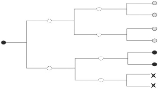
Diagram representing artificial cell lineage tree where light grey cells are positive definite, black cells are negative definite, the X shape cells are dead cells and the white ones, with dashed contour, are unobservable.

Open in new tabDownload slide

Without any supplementary prior information the VB approach proved to be superior to the ML method. The ML approach obtains a single estimate of the HMT model parameter, whereas the VB-HMT obtains a posterior distribution for the HMT model parameters. The VBS-HMT model performed better than the VB-HMT model based on the original upward–downward algorithm. As shown in Table 1, the estimated values of parameters θ_VBS−HMT is closer to the values of true parameter θ compared with θ_ML+P or θ_VB−HMT, i.e. the error and relative entropy for the VBS–HMT model are smaller.

At the testing step, we made use of the second set of 30 artificial lineage trees which were obtained using the same set of parameters θ used for generating the training set.

For the performance comparisons of the four models, at the testing step, we need to determine the percentage of correct predicted states of nodes.

Let

(24)

and

(25)

The trained models were applied to the testing set and the 𝒫 calculated for all four models. In Figure 3, we compare the performances of the four algorithms, varying the size of the training data. The aim here is to predict the unobserved cell type at all levels within each lineage tree in the test set as accurately as possible. From this figure it can be seen that, for the largest training set the models predicted the types of cell at all levels with high accuracy. The ML-HMT had the poorest performance. VB-HMT and the ML-HMT with supplementary prior information had similar behaviour and are superior to the simple ML approach. VBS-HMT had the best performance compared with the previous two models mentioned above. The VBEMS estimates obtained from the set of 30 stem cell lineage trees were very good as the produced posterior distributions are tight distributions (see Supplementary Material) and because the estimation of the full posterior captures most of the model uncertainties as opposed to a point estimate of the model-parameter posterior in the ML case. The use of synthetic data permitted a true test of the models since the information on the types of cells at all cell division levels within each lineage tree are known. For real lineage trees, such cell-type information at intermediate levels are generally unknown. It is to be noted that the resulting VBEMS algorithm generalizes the standard EM algorithm and its convergence is guaranteed (Attias, 2000; Beal and Ghahramani, 2003). The computational cost for the VB with smoothed probabilities approach is of the same order to that of the ML approach (Dasgupta and Carin, 2006).

Fig. 3.

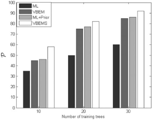
Model prediction performance with varying amounts of training data. Three blocks of bar diagrams have been produced showing the performance of the ML-HMT, VB-HMT, ML+P-HMT and VBS-HMT for a different size of training dataset: 10, 20, 30 lineage trees. The vertical axes shows the percentage of predicted cells type that have been right.

Open in new tabDownload slide

After model validation and comparison to other models in the literature using synthetic data, we applied the VBS-HMT model to the real stem cell lineage trees. The outcome of the time-lapse experiment consists of a dataset of 30 stem cell lineage trees in which the expression of SSEA3 can only be observed at the leaf and the root levels, i.e. x₁ and x_leaf are known. We estimated the model parameters θ = [π, vec(P), vec(C)]^T using the VBEMS algorithm applied to the set of incomplete lineage trees. Subsequently, we predicted the presence or absence of SSEA3 expression at the unobserved positions within the trees, see Figure 4. In the biological context, π represents the probabilities of the root cell to be in one of the three possible states, i.e. SSEA3^Positive, SSEA3^Negative and dead, P_ij expresses the probabilities of transitions from one of the possible states to another and C_jh expresses the probabilities of a cell of a particular state to be true stem cell, differentiated cell or dead cell. In several lineage trees, our model predicted that SSEA3^Negative cells give rise to SSEA3^Positive progeny. This suggests that NTERA2 stem cells could regain SSEA3 expression, i.e. the transition from SSEA3^Negative to SSEA3^Positiveis possible. This transition event has been validated by the real stem cell experiment in which a percentage of the root cells that were SSEA3^Negative stem cells produced SSEA3^Positive progeny.

Fig. 4.

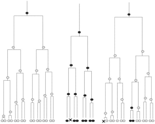
Diagram representing experimental stem cell lineage trees where light grey cells at the leaf level are observed positive definite, black cells at the root and the leaf levels are observed negative definite, the X shape cells are observed dead cells, the light grey cells at the intermediate levels are predicted SSEA3^Positive cells, and the black cells at the intermediate levels are predicted SSEA3^Negative cells.

Open in new tabDownload slide

Our proposed model, VBS-HMT, enables interpretation of data from real-time single cell analysis. Combining time-lapse analysis of single cells and the VBS-HMT model, it is possible to predict the unvisualized event of SSEA3 negative cells converting to the SSEA3 positive state. The VBS-HMT model predicts that the conversion of SSEA3 negative cells to the SSEA3 positive state occurs prior to the first cell division in 35% of cases. Culture conditions and numerous compounds affect the stability of cell populations, either inducing cell differentiation or stabilizing the cell population in its current state. Determining the kinetics and probability with which cells fluctuate between discrete states is important for understanding the physical properties of cells. Resolving this with the use of single cell analysis helps to identify if a cell population is functionally homogeneous or consists of different cell types. This information can in turn be used to more accurately direct the differentiation of stem cells to desired cell types. Utilization of the VBS-HMT model is not confined to the study of stem cell populations but can prove useful in the study of lineage selection during cell differentiation. Given data from a time-lapse analysis, the VBS-HMT model can help to predict when differentiating sister cells and progeny diverge with respect to cell type (i.e. mesoderm versus ectoderm).

Overall, the model enables us to predict decision events which are difficult to visualize. The results of the model simulations can then be used to generate testable hypothesis.

7 CONCLUSIONS

In this article, we developed the VBS-HMT model and applied it to incomplete tree structured data. The model proved to be superior to other models in the literature when tested on the prediction of the type of cells at each division level within a lineage tree as well as on the estimation of model parameters. We succeeded in confronting the underflow problems by combining the variational Bayesian method with the upward–downward algorithm with smoothed probabilities as an E-step in the EM context. The resulting algorithm was demonstrated to have superior performance over the competing approaches and was applied to the real stem cells lineage modelling problem. The VBS-HMT model provides the means to objectively predict a cell's phenotype from knowing the phenotype of the cells at the root and leaf level within the cell lineage tree. It is important to note that the proposed inference algorithm is able to predict novel behaviours based on incomplete data, which are not directly observable. These predictions can subsequently be validated by targeted experiments

Funding: Engineering and Physical Sciences Research Council (EPSRC).

Conflict of Interest: none declared.

REFERENCES

Author notes