Correlating multiple SNPs and multiple disease phenotypes: penalized non-linear canonical correlation analysis

Abstract

1 INTRODUCTION

Complex diseases are caused by a combination of environmental and genetic factors, which by themselves cannot cause the disease. Contrary to monogenetic diseases, complex diseases have no clear-cut pattern of inheritance; therefore, the number of suspected genes may be large. Finding the relevant genes out of a large number of suspicious genes is difficult, especially since the expression of genes are regulated in complex pathways that are influenced by many extra- and intracellular factors. Among the latter are expressions of other genes, gene copy numbers and single nucleotide polymorphisms (SNPs). By associating multiple datasets containing information about a patient's phenotypic and genetic details, common features can be captured and an underlying genetic background of the complex disease (i.e. its molecular mechanism) will be revealed.

Canonical correlation analysis (CCA; Hotelling, 1936) is a commonly known method to study the association between two (or more) sets of variables, it finds linear combinations of all the variables in one set which correlate maximally with linear combinations of all the variables in the other set(s). CCA can be used to study the idea that variations in SNPs can have an effect on the expression of multiple genes and vice versa changes in gene expression levels can be caused by variations in multiple SNPs; i.e. it can reveal information about networks of co-expressed and co-regulated genes and their associating SNPs.

Previously, we have shown that adapting the elastic net (Zou and Hastie, 2005) to CCA, and reducing it to univariate soft-thresholding (UST), makes the interpretation of the CCA results easier by extracting only relevant variables out of high-dimensional datasets (Waaijenborg et al., 2008). This so-called penalized CCA makes sure that the information loss is minimized while keeping the predictive performance high. Highly correlated variables, caused by, e.g. co-expressed genes, are grouped into the same results. Furthermore, it handles data in which the number of variables exceeds the number of subjects by far. Unfortunately, when one or both of the datasets contain variables measured on a qualitative scale, the nature of the data is ignored by CCA and each variable is supposed to have an additive effect on the succeeding categories.

SNPs are frequently used genetic data, that have a qualitative nature. For each SNP there are three possible genotypes: (i) wild-type, for the common allele, (ii) heterozygous and (iii) homozygous, for the less common allele; usually coded as 0, 1 and 2, respectively. When the qualitative nature of the SNP data is ignored, each SNP is supposed to have an additive effect. Optimal scaling transforms each SNP variable into a quantitative variable while accounting for its characteristics, so differences can be made between SNPs with an additive, dominant, recessive and no effect. CCA with optimal scaling was introduced by de Leeuw et al. (1976) and further refined by van der Burg and de Leeuw (1983; 1987); this so-called non-linear CCA relates two (or more) sets of non-linearly transformed variables in an optimal way.

Like with all regression methods, in the presence of multicollinearity the parameter estimates of optimal scaling in regression are unstable (Buja et al., 1989; Morlini, 2006). Multicollinearity can be caused by, e.g. neighboring SNPs (forming haplotypes); these highly correlated SNPs are said to predict the outcome of one another and other nearby sites. It is sometimes suggested to eliminate all SNPs except one, out of a group of highly correlated SNPs; however, preprocessing the data and making decisions about which SNP to select are obscure, it is better to find a method which automatically groups highly correlated SNPs into the same results. This is achieved by combining the penalized CCA with non-linear CCA; the variable selection in penalized CCA can be performed such that highly correlated variables are grouped together.

In this article, we describe a penalized non-linear CCA (PNCCA) approach for quantifying the association of the expression levels of multiple genes with multiple SNPs, such that it accounts for the qualitative character of the SNP data by estimating the quantification of the genotypes. Soft-thresholding is used as a penalty function to limit the number of gene expressions and the number of SNPs, resulting in more interpretable results. By means of simulation studies, we illustrate that our approach is capable of identifying groups of genes and SNPs—out of a large set of variables—that are truly associated. Finally, we present an application of our method on genetic data of 144 patients with glial cancer (Kotliarov et al., 2006).

2 METHODS

Our objective is to extract groups of variables that capture common features, out of two large sets of variables, one containing information about the disease phenotypes, for instance, a set of gene expression values, and the other containing SNP information, obtained from a sample of patients. Therefore, we adjust classical CCA such that it can extract groups of highly correlated variables; consequently, co-regulated/co-expressed genes in a pathway and associating haplotypes in a gene are maintained. This is achieved by introducing a penalty function in CCA. Furthermore, our adjusted CCA is capable of handling qualitative and quantitative variables.

First, we introduce a way to solve CCA such that adaptations can be easily made; we show how penalized CCA is performed and adapt this for qualitative data. Finally, we describe methods to determine the optimal penalty parameter. Sections 2.1 and 2.2 summarize the penalized CCA presented in our previous paper (Waaijenborg et al., (2008), for more details of the method we refer to this article.

2.1 Canonical correlation analysis

Consider the n × p matrix Y, containing p (gene expression) variables and the n × q matrix X, containing q (SNP) variables, obtained from n individuals. CCA tries to find linear combinations of all the variables in Y which correlate maximally with linear combinations of all the variables in X. These linear combinations are the so-called canonical variates ω and ξ, such that ω = Yu and ξ = Xv, with the weight vectors u' = (u₁,…, u_p) and v' = (v₁,…, v_q). The optimal weight vectors are obtained by maximizing the correlation between the canonical variate pairs, also known as the canonical correlation.

By converting the CCA problem into a regression framework, adaptation of penalization methods will become easier. This conversion can be obtained by the two-block Mode B of Wold's original partial least squares (PLS) algorithm (Wold, 1975; Wegelin, 2000). Wold's algorithm is an iterative process that begins by estimating an initial canonical variate pair based on an initial guess of the weights assigned to the original variables. The objective is to maximize the canonical correlation, therefore, the initial canonical variate pair ξ and ω are regressed on, respectively, Y and X to estimate a new set of weights. With this new set of weights, a new pair of canonical variates is determined, which are in turn regressed on Y and X. This process is repeated until the weights converge, resulting in the first pair of maximally correlating canonical variates. Hereafter, the residual matrices of Y and X are determined and the algorithm is repeated for the residual matrices to obtain the remaining pairs of canonical variates. This process can be repeated until the residual matrices contain no more information or until the decision is made that further analysis is no longer useful.

Since Wold's algorithm performs two-sided regression (one for each set of variables); either of the two regression models can be replaced by another method for optimizing the weight vectors; such as one-sided penalization or different penalization methods for either set of variables. In this article, we will transform and penalize the SNP variables (X-side) and penalize the gene expression variables (Y-side).

2.2 Penalized CCA

Previously, we proposed penalized CCA (Waaijenborg et al., 2008), where we performed the same penalization method on both sets of variables. UST (Zou and Hastie, 2005) was used to penalize, since it solves general problems which arise when dealing with microarray studies, such as multicollinearity due to co-regulated and co-expressed genes, and overfitting caused by the small number of subjects and the large number of variables. Furthermore, reduction of the large number of variables within the canonical variates can be obtained, such that interpretation of the results becomes easier.

The estimation of the weight vector for the gene expression variables is as follows:

with f₊ = f if f > 0 and f₊ = 0 if f ≤ 0, and λ the penalty parameter. Because UST disregards the dependency between variables within the same set, the grouping effect is maintained. The optimal penalty parameter can be chosen based upon the cross-validation tests (see Section 2.6). This penalization method can be applied to quantitative variables; when applied directly to qualitative variables, the underlying nature of the variable may be ignored.

Parkhomenko et al. (2007; 2009) suggested a similar penalized CCA method. Witten et al. (2009) discussed penalized CCA in a general framework of sparse matrix decomposition methods.

2.3 Optimal scaling procedure

CCA was first applied to quantitative variables, and non-linear CCA made it possible to associate two sets of qualitative variables (Young et al., 1976; van der Burg and de Leeuw, 1983). Non-linear CCA alternates back and forth between two phases (alternating least squares), one which determines the canonical weights and transformations for one set, while keeping the other set fixed, and vice versa. Since only the set with SNP variables (X) contains qualitative variables, only this set has to be transformed. To accomplish this we have to alter Wold's algorithm, such that set X is transformed in such a way that the linear combinations of the original set Y and the transformed set X correlate maximally.

By making use of optimal scaling (Young et al., 1976; van der Burg and de Leeuw, 1983), each qualitative SNP variable is transformed into one continuous variable, that is, variable x_j is related to variable x_j^* by a transformation which completely satisfies the measurement characteristics of the SNP data. That is,

where ℑ_j are the measurement transformations for variable j, which are subjected to restraints by the measurement level (i.e. nominal, ordinal or interval).

Each SNP has three possible genotypes: (i) wild-type (the common allele); (ii) heterozygous; and (iii) homozygous (the less common allele). These genotypes can have an additive, dominant, recessive or constant effect; this knowledge determines the ordering of the corresponding transformed variables. The restricted ordering

(with a: wild-type, b: heterozygous and c: homozygous) captures all the possible transformations of each SNP. It indicates that the effect of the heterozygous form of SNP j always lies between the effect of the wild-type and homozygous genotype. If before restriction, the effect of the heterozygous genotype exceeds or lies beneath the effects of the wild-type and the homozygous genotype, the heterozygous category is merged with the genotype whose effect is most similar.

The possible transformations are as follows:

With these restrictions in mind, optimal scaling within CCA is done as follows. Consider the n × q matrix X, containing q SNP variables, obtained from n individuals and the response variable ⁠, the estimated canonical variate of the gene expression data. Let G_j be the n × g_j indicator matrix for variable j (j∈(1,…, q)), with g_j the number of categories of variable j. And c_j the categorical quantifications of variable j. Then the optimal scaling algorithm [based on the CATREG algorithm (van der Kooij, 2007)] will look as follows:

1. Normalize the data, such that mean(G_jc_j)=0 and c_j′G_j′G_jc_j=n. And and ⁠.

2. Set starting values and z = ∑_j=1^qv_jG_jc_j.

3. Transform X into X^*, as follows

   Repeat loop across variables  j, j = 1,…, q

   • Remove contribution variable j from zz_j=z−v_jG_jc_j

   • Obtain unrestricted transformation of c_j

   • Restrict and normalize to obtain c_j^*

   • Update v_j

   • Update zz = z_j+v^*_jG_jc^*_j

   until v has converged.

The algorithm optimizes each variable at a time, such that the transformed variable explains the part of the outcome ω which is not explained by the other (transformed) variables. As the variable is optimally transformed, it is restricted to the ordering as given above. Hereafter, the next variable is optimized and so on, until the algorithm converges.

As with all regression models, the parameter estimates of this algorithm may be unstable in case of multicollinearity. Van der Kooij (2007) implemented the elastic net (Zou and Hastie, 2005) into the CATREG algorithm, thus combining the elastic net with optimal scaling, such that multicollinearity no longer forms a problem and built-in variable selection can be performed. It operates the same as the optimal scaling algorithm given above, only the updated v^*_j's (Step 3d) are penalized following the equation:

The elastic net contains two penalty parameters, namely the lasso (Tibshirani, 1996) and the ridge penalty. Here, the soft-thresholding (numerator) takes care of the lasso penalty (λ₁) and then a proportional shrinkage for the ridge penalty (λ₂) is applied (denominator). After convergence, the weight vector v^{*_{elastic net}} is multiplied with (1 + λ₂) to prevent double shrinkage.

To reduce the computation time, we set the ridge penalty to infinity, which in the elastic net as proposed by Zou and Hastie Zou and Hastie (2005) for quantitative variables results in UST. From Van der Kooij's algorithm, we can see that by setting the ridge penalty to infinity, the contribution of each updated variable is so small that the updated z reduces to zero (Step 3e) and the transformation only depends upon ⁠, resulting in univariate transformations. Thus, we ignore the effects of all the other variables and transform each variable separately based upon ⁠, such that highly correlated variables transform similarly and get similar weights.

2.4 PNCCA

Combining the penalization method and the penalized optimal scaling method, results in the following PNCCA algorithm (also depicted in Fig. 1):

1. Standardize Y and X.

2. Set k ← 0.

3. Assign arbitrary starting values and ⁠. For instance, set and ⁠, such that |cor(x_r, y_s)| = max(|cor(x_j, y_i)|), with r∈(1,…, q), s∈(1,…, p), j = 1,…, q and i = 1,…, p.

4. Estimate ξ, ω, v and u iteratively , as follows

   Repeat  

   • k ← k+1.

   • and (with and as given in Step 3).

   • Obtain the transformed matrix X^* by minimizing the distance between and X. That is,

     

     with G_j the n × g_j indicator matrix for variable j with g_j, the number of categories of variable j.

     Restrict to obtain c^*_j. Then x^*_j = G_jc^*_j.

     Standardize X^*.

   • Compute and û^(k) with UST.

     

     with f₊=f if f>0 and f₊=0 if f≤0.

   • Normalize and û^(k).

    until   and û^(k) have converged.

Fig. 1.

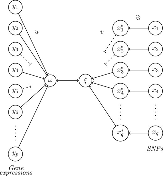
The PNCCA. Qualitative variables within dataset X are transformed (ℑ) (based upon ω) into quantitative variables (X^*). Datasets Y and X^* are summarized into underlying structures (ω and ξ), which correlate maximally. Variables that contribute little, based upon their weights (u and v) are eliminated (dotted lines) and the relevant variables remain.

Open in new tabDownload slide

2.5 Residual matrices

It is unlikely that in large genomic datasets, all associations can be explained by one single canonical variate pair. Therefore, it might be useful to look for additional information contained in the datasets. A second pair of canonical variates can be obtained through the residual matrices of X and Y; therefore, the part of the variables that explain the first pair of canonical variates is removed from the sets. It has been shown for PLS that as long as either of the two residual matrices is determined the results remain the same (Lindgren and Rännar, 1998); since CCA can be seen as a special case of PLS (Wegelin, 2000), we only determine the residual matrix for Y.

To show that only one of the X or Y matrices needs to be deflated, we have to prove that X^(r+1)'Y^(r+1) = X^(r)′Y^(r+1) = X^(r+1)′Y^(r) (Dayal and MacGregor, 1997). Let γ_jξ be the part of ξ explained by variable x_j, and θ_iω the part of ω explained by variable y_i. Then

(ξ′ω) is a scalar which equals the canonical correlation and since ξ′Y=(θ(ξ′ω))′, it follows

Further canonical variate pairs can be obtained in similar way, until the residual matrix contains no more information or until the decision is made that further analysis is no longer useful.

PNCCA only gives a small number of gene expression variables a non-zero weight, therefore, only the residuals of these variables have to be determined. Additionally, to make sure that each SNP variable can only be transformed once in an optimal way, we fix the SNP variables that get a non-zero weight, in their primary transformed form, while estimating additional pairs of canonical variates.

2.6 Optimization of penalty parameters

Optimization of the penalty parameters for each canonical variate pair is determined by k-fold cross-validation. The dataset is divided into k subsets (based upon subjects), of which k − 1 subsets form the training set and the remaining subset forms the validation set. The weight vectors u and v and the transformation functions ℑ_j are estimated in the training set and are used to obtain the canonical variates in the training and validation sets. This is repeated k times, such that each subset has functioned both as a validation set and part of the training set.

Instead of determining the penalty, it is for sake of interpretation and to reduce computation time easier to determine the number of variables to be included in the final model. This approach is also used by Lê Cao et al. (2008) and Shen and Huang (2008). We determined within each iteration step, the penalty parameter that corresponded with the selection of the predetermined number of variables and penalized accordingly. We determined the optimal number of variables within the two sets. Five possible optimization criteria were investigated (see Section 3.1). The first criterion minimized the mean difference between the canonical correlation of the training and validation sets (Waaijenborg et al., 2008);

However, this optimization criterion has a drawback since the canonical correlation of the validation set can change sign with respect to the canonical correlation of the training set. This would mean that if the canonical correlation of the validation set changes sign it would not be penalized more than when the sign would not change. Therefore, a better optimization criterion should minimize the following

Parkhomenko et al. (2009) proposed to determine the penalty parameters by maximizing the mean absolute canonical correlation of the validation sets;

This criterion also does not keep the possible sign change into account and could be better replaced by

Previously, we proposed (Waaijenborg and Zwinderman, 2007) to evaluate the predictive performance of the canonical variates of the training set by minimizing the mean squared prediction error (MSPE) of the canonical variates

Here, and û^−j are the weight vectors estimated by the training sets, X^*_−j and Y_−j in which subset j was deleted and X^*_j the transformed validation set following the transformation of the training set X^*_−j. and û>_−kj are the weights estimated by the training sets in which subject j was not present. By varying the number of variables within the set of gene expression variables and the set of SNPs, the optimal number of variables within each set which minimize or maximize (depending on the criteria) the different criterion is determined.

2.7 Permutations

If the number of variables is large, there is a high probability that a random pair of variables has a high correlation by chance, while in the population there is no correlation. Because the canonical correlation is at least as large as the largest observed correlation between a pair of variables, the canonical correlation can be high by chance as well. To identify a canonical correlation that is large by chance only, we performed a permutation analysis on the validation sets. We permuted the canonical variate ξ (SNP profile) and kept the canonical variate ω (gene expression profile) fixed and then determined the difference between the canonical correlation of the training and the permuted validation sets; this was compared with the difference between the canonical correlation of the training and of the non-permuted validation sets. The closer they are together, the higher the chance that the model does not fit well.

2.8 Data

Adult gliomas are a lethal group of brain tumors, persons with certain SNP profiles might be at higher risk of developing these tumors. PNCCA can be used to investigate the effect of these SNP profiles on gene expressions, and so identify networks of co-expressed and co-regulated genes associated with the progression of glioma.

Gene expression levels together with SNP data of 144 human gliomas of various tumor grades and histogenesis [24 astrocytomas (7 grade 2 and 17 grade 3), 46 oligodendrogliomas (34 grade 2 and 12 grade 3) and 74 glioblastomas] were collected, as described by Kotliarov et al. (2006). These two sets contained expression levels of 54 613 genes (HG-U133 Plus 2.0) and the data on 53 346 SNPs (XbaI-restricted DNA), situated in the autosomal and sex-linked chromosomes. SNPs with >20% missing data and monomorphic SNPs were deleted, further missing data were imputed. Since we were not interested in rare SNP profiles, we did not allow for SNP categories with <5% observations, and therefore merged them with adjacent categories. The gene expression data were log2 transformed.

3 RESULTS

3.1 Simulation

To investigate if penalized non-linear CCA is able to extract relevant variables out of large datasets and to determine which optimization criterion performs best, we performed 100 simulation studies. One pair of canonical variates was simulated, existing of 20 SNP variables and 30 gene expression variables. Irrelevant variables were added to the sets such that the SNP set contained 1000 variables and the gene expression set contained 2000 variables, measured in 10 differing number of subjects (10 simulation studies per sample size).

For each simulation set, continuous variables were generated. The absolute maximum correlation between the sets was between 0.40 and 0.65, and within the sets between 0.33 and 0.66. One part of these variables were transformed into SNP variables, where nine SNPs were additive, eight SNPs were dominant or recessive and three SNPs contained only two categories. Irrelevant SNPs were generated through sampling out of a real set of SNP variables, SNP variables were randomly selected and permuted over the subjects. Irrelevant gene expressions were drawn from a normal distribution with mean zero and a SD of one. We performed 10-fold cross-validation, while searching through a 100 × 100 variable grid; we took steps of 10 variables per set while keeping the number of variables of the other set fixed, and vice versa; resulting in 100 variable set combinations. This was done to evaluate the optimal number of variables within the canonical variates pairs given by the different optimization criteria (as described in Section 2.6) and for different sample sizes (Fig. 2).

Fig. 2.

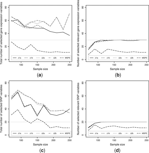
The optimal number of variables based upon the different optimization criteria (as given in Section 2.6). (a) The total number of selected gene expression variables, (b) the number of selected gene expression variables out of the ‘true’ dataset, (c) the total number of selected SNP variables and (d) the number of selected SNP variables out of the ‘true’ dataset. The gray lines represent the number of ‘true’ variables in the simulated datasets.

Open in new tabDownload slide

Figure 2 shows the effect of the sample size on the total number of selected variables (Fig. 2a and c), and on the number of selected variables out of the simulated canonical variate pairs (Fig. 2b and d), i.e. the number of relevant variables. The criteria that minimized the difference between the canonical correlation of the training and validation sets (△_cor^1a and △_cor^1b) and the criteria that maximized the canonical correlation of the validation sets (△_cor^2a and △_cor^2b) overestimated the optimal number of variables. The larger the sample size, the smaller this overestimation and the closer the optimal number of variables approached the true number of relevant variables, 30 gene expression variables (Fig. 2a) and 20 SNP variables (Fig. 2c). The criterion that minimized the MSPE underestimated the optimal number of variables, especially in the case of the gene expression variables (Fig. 2a).

As the sample size increased, all criteria were more accurate at selecting the relevant variables (Fig. 2b and d). The MSPE criterion was the most accurate one, by selecting almost only relevant variables. However, MSPE underestimated the number of relevant variables, thereby missing around half of the relevant variables.

Overall the first two minimization criteria (△_cor^1a and △_cor^1b) seemed to do better in reducing the number of selected irrelevant variables; especially when the sample size increased, compared with the maximization criteria (△_cor^2a and △_cor^2b). There was no substantial difference between the optimization criteria that did not keep the possible sign change of the canonical correlation of the validation set into account and those who did penalize for it. We chose to base all further optimizations upon criterion △_cor^1b.

For the purpose of illustration, we also performed PNCCA on a dataset containing two pairs of simulated canonical variates. These canonical variates were simulated as described above, with one pair containing 20 SNPs and the expression levels of 30 genes and the second pair containing 30 SNPs and 30 genes, measured in 140 subjects.

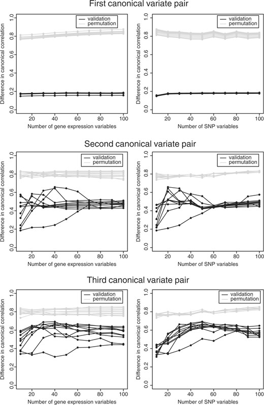
We divided the dataset into two sets, a test set containing 40 subjects and another set containing 100 subjects. On the latter, we performed 10-fold cross-validation on the same grid as described before, to determine the optimal number of variables within the canonical variates pairs (Fig. 3) and the optimal number of pairs. Figure 3 shows the effect of the choice of the number of variables for the canonical variate pairs on the difference in canonical correlation between the training and the validation set. Adding variables to the canonical variate pairs, had little effect on the difference in canonical correlation. Only for small numbers of variables we saw an improvement in the effect of adding variables, i.e. the difference in canonical correlation decreased. The optimal number of variables in the first canonical variate pair were 50 SNP and 50 gene expression variables. We applied these penalties to the full cross-validation set of 100 subjects to obtain the weights and the transformations and employed these to the test set. The cross-validation set had a canonical correlation of 0.947 and the test set had a canonical correlation of 0.917. Almost all the selected variables were variables out of the second simulated canonical variate pair (one relevant SNP variable was not selected), with some additional irrelevant variables in both sets. Figure 4 shows how the additive, dominant and recessive SNP variables were transformed, it can be seen that the dominant and recessive SNPs do not always clearly reflect dominance or recessiveness (Fig. 4b). For example, the recessive effects (gray lines) mostly show that the homozygous and heterozygous mutant have the same effect; however, there are two variables that show an additive effect (shown by the straight downward going line). For the dominant SNPs, there is one SNP that shows an additive effect (straight upward going line).

Fig. 3.

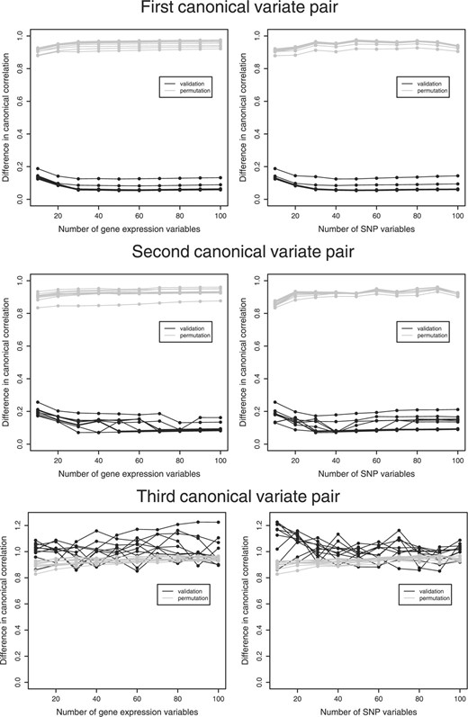
Simulation study. The effect of the choice of the number of variables without zero weights in the penalty on the mean difference in canonical correlation between the training and the validation set (black) and the training and the permutation sets (gray) for three succeeding canonical variate pairs. Each line represents the effect of the number of selected variables in that set, while the number of selected variables in the other set stays fixed. In the right column the effect of the number of SNP variables and in the left the effect of the number of gene expression variables.

Open in new tabDownload slide

Fig. 4.

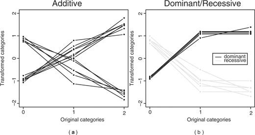
The transformation for the SNPs in the first canonical variate. (a) the transformation of the additive SNPs and (b) the transformation of the dominant (black) and recessive (grey) SNPs.

Open in new tabDownload slide

The optimization of the number of variables for the second canonical variate pair showed similar results (Fig. 3). This canonical variate pair optimized at 30 SNP and 40 gene expression variables with a canonical correlation of 0.918 in the full cross−validation set and 0.861 in the test set, with all variables out of the first simulated canonical variate pair, with some additional irrelevant variables in both sets. Results of the transformed SNPs were comparable with those from the first obtained canonical variate pair (data not shown).

Whereas the cross-validation results of the first two pairs were non-overlapping with the permutation results, the results for the third canonical variate pair clearly overlapped (Fig. 3). Thereby, we concluded that no further relevant information was present in the residual matrices.

3.2 Glioma data

Due to the high computation time that is necessary to obtain the optimal number of variables via 10-fold cross-validation over a grid of 100 × 100 variables, we analyzed these data per chromosome and present the results of one chromosome, namely chromosome 17. This chromosome exists of 898 SNP variables and 2893 gene expression variables. Subjects were divided into two sets, one test set containing 44 subjects and a set of 100 subjects was used in the optimization of the model. Optimization of the number of variables was determined by criterion △_cor^1b. From Figure 5, it can be seen that the criterion is minimized for a canonical variate pair with 10 gene expression variables and 10 SNP variables. Adding more variables to the canonical variates did not give an improvement.

Fig. 5.

Glioma data. The effect of the choice of the number of variables without zero weights in the penalty on the mean difference in canonical correlation between the training and the validation set (black) and the training and the permutation sets (gray) for three succeeding canonical variate pairs. Each line represents the effect of the number of selected variables in that set, while the number of selected variables in the other set stays fixed. In the right column, the effect of the number of SNP variables and in the left the effect of the number of gene expression variables.

Open in new tabDownload slide

In determining whether more information was contained in the remainder of the data, we looked for two additional canonical variates, via the residual matrices. From Figure 5, it is clear that as the number of variables increased, the difference in canonical correlation increased. Thus, smaller number of variables within the canonical variates resulted in more stable results. The second canonical variate pair contained 10 gene expression variables and 10 SNPs, the third canonical variate pair contained 40 gene expression variables and 10 SNPs. The canonical correlation of the first three pairs were 0.802, 0.756 and 0.805, and the canonical correlations of the test set 0.845, 0.480 and 0.080, respectively.

As we optimized the succeeding canonical variate pairs (Fig. 5), the results of the optimization criterion approached the results of the permutation more and more; indicating that the results became less prominent as the number of canonical variate pairs increased, this is also shown by the lowering canonical correlation of the test sets.

The location of the obtained SNPs and genes within chromosome 17 is shown in Figure 6, it shows that especially for the first canonical variate pair, a large part of the SNPs and genes that were highly associated were also closely located on the chromosome. This is to be expected, since structural alterations within or close to a gene are more likely to influence a gene's expression.

Fig. 6.

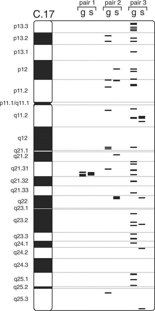
Location of the selected genes and SNPs in chromosome 17, g represent the selected genes and s the selected SNPs. From left to right, the first, second and third canonical variate pair is depicted.

Open in new tabDownload slide

4 DISCUSSION

SNPs are known to be associated with phenotypic variations (Stranger et al., 2007). By associating the expression levels of multiple genes with multiple SNPs, underlying genetic backgrounds, e.g. complex diseases can be revealed.

Standard multivariate analysis methods are too restricted in the number of variables they can handle. Additionally, they cannot handle variables measured on a qualitative scale, and ignore the underlying structure of this data. Parkhomenko et al. (2007) and Waaijenborg and Zwinderman (2007) associated SNP variables with gene expression variables, using a sparse version of CCA. Parkhomenko et al. (2007) took account of the family structure present in the data. Waaijenborg and Zwinderman (2007) transformed each SNP variable into two dummy variables, thereby doubling the number of variables and thus the computation time. No restrictions were made about the nature of the SNP variables, in either of the two studies.

By adapting UST and optimal scaling to CCA, we obtained a tool to extract relevant associating variables out of high-dimensional datasets, without destroying the underlying structure of the data. It worked well in cases where the number of variables highly exceeded the number of subjects.

The CANALS method (van der Burg and de Leeuw, 1983) performs CCA with optimal scaling. The elastic net and/or UST can also be applied to this method. CANALS estimates the optimal weights and the optimal transformations for several canonical variate pairs at once, such that each categorical variable is transformed in one overall way that is optimal for all canonical variate pairs. However, our implementation of this method increased computation time by a factor 50 (for only two pairs of canonical variates), so we preferred the residual approach although it has the downside that for pairs of canonical variates after the first, the transformations might be suboptimal. Another downside of this method is that only one set can contain categorical variables.

In large genomic studies like this one, fixation of previously transformed SNPs is optional when obtaining additional canonical variates. There is so much information in the dataset and so many different phenotypes (formed by combinations of gene expression variables), that there is almost no overlap between the obtained results; there is no overlap between the selected variables in the different canonical variate pairs. For smaller studies, where one of the two sets of variables will not be penalized, fixation of the transformed SNP variables is recommended.

Computation time is still a big burden in genome-wide studies, and also in our study. An advantage of our approach is that one may consider the joint SNP effects on multiple chromosomes simultaneously. However, due to computation time, we decided to analyze the data per chromosome. Moreover, in our grid search, we took steps of 10 variables, a much more refined grid could reduce the number of irrelevant variables, but would increase the computation time tremendously. Refining the search around the place of interest will further refine the analysis.

Although the PNCCA worked well when the number of variables exceeded the number of subjects, from simulation studies it can be seen that the number of subjects in the validation set should not be too small. We showed that as the number of subjects increased, the precision increased; i.e. the number of selected irrelevant variables decreased and the number of selected relevant variables increased.

In this article, we mainly focused on SNP variables, where the characteristics of the SNP variables were maintained and we observed what genetic effect they had, i.e. dominant, recessive or additive. Our PNCCA can also be applied to other categorical data, such as haplotype data and genetic markers with more than three categories, but then different restrictions have to be applied during the optimal scaling step in the algorithm.

Because the penalty parameters are already present in the first step of the algorithm, they have some influence on the variables chosen in that step and therefore have large influence on which variables stay in the proceeding steps of the algorithm. The choice of starting values is therefore important; we decided to choose the two variables that had the maximum between subset correlation as the starting values. This method does not always obtain the highest canonical correlation, or a decreasing canonical correlation in the succeeding canonical variate pairs, but our experience with this choice is positive.

To determine the optimal number of variables within each canonical variate, we compared five different optimization methods. The model obtained from the training set should be as representative as possible for the validation set, and thus the canonical correlation should be as similar as possible. Therefore, by only looking at the canonical correlation of the validation sets, the results of the training set are ignored. We also see that in such cases the optimal number of variables is overestimated, since irrelevant variables can make a positive contribution to the canonical correlation.

Daye and Jeng (2009) show the poor predictive performance of UST compared with other penalization methods, including the lasso and the elastic net. Their focus lies on the predictive performance of the model and not on variable selection. According to the results in Tables 2 and 4 in their paper, UST performs variable selection quite well. Moreover, their simulation studies consists of situations where p < n, while our focus lies in p > > n, in which case UST seems to perform well (Tibshirani, 2009).

PNCCA can be seen as a first tool to investigate complex diseases by obtaining groups of suspicious genes and SNPs that are highly associated. Further biological modeling can then be performed on a much reduced dataset.

Funding: Netherlands Bioinformatics Centre (NBIC).

Conflict of interest: none declared.

REFERENCES

Author notes