Efficiently finding genome-wide three-way gene interactions from transcript- and genotype-data

Abstract

1 INTRODUCTION

We address the issue of efficiently finding a three-way gene interaction, precisely two interacting genes in expression under the genotypes of a different gene, given a dataset in which both gene expressions and genotypes are measured for each individual. We illustrate our problem setting by using synthetic 2D diagrams in Figure 1, where expression values of two genes are plotted with three classes (genotypes): +, * and △. In this figure, panel (a) shows expression values being just randomly distributed; (b) shows expression values being easily categorized into three classes; and (c) shows that classes can be categorized by expressions without using two genes at the same time. We are not interested in (a–c) but in (d), which shows that the correlation in expression between two genes differs for each class. More concretely, two genes are positively correlated for one class, whereas they are negatively correlated for another. This is exactly a switching mechanism in expression between correlation and inverse-correlation of two genes, controlled by another gene. Also this is the three-way gene interaction which we attempt to find in this article. We note that this can be categorized into a general switch in biology. A simple, well-known example is Max, a transcription factor, which plays a role of an activator or a suppressor, depending on whether it binds to Myc (i.e. Myc-Max) or Mad (i.e. Mad-Max) (Ayer and Eisenman, 1993). We emphasize that this type of interaction must be a key to elucidating complex biological systems.

Fig. 1.

Synthetic examples: expressions of two genes under the three classes of another gene. (a) randomly distributed, (b,c) easily categorized into three classes and (d) a switching mechanism.

Open in new tabDownload slide

A reasonable approach to detect such three-way interactions is the likelihood ratio test for regression (LRTR). Particularly, logistic regression must be suitable the most, because of categorical responses (genotypes) in our setting (McCullagh and Nelder, 1989). The first item of note is that parameter estimation for logistic regression is based on the maximum likelihood, for which a time-consuming iterative gradient descent, Newton–Raphson, is usually used. Secondly, in our case, classes are genotypes, causing a problem of an explosive number of combinations of one SNP (genotypes) and two genes (expressions). For example, for 50 000 SNPs and 1000 genes, we have roughly 5 × 10¹⁰ (= 50 000 × 1000 × 1000) combinations, making scanning over all possible combinations intractable. In fact, >24 h are needed to run Newton–Raphson over only 10⁷ combinations in our experiments. Thus, the main focus of this article is to speed up the procedure of finding the three-way interactions. Our strategy for this issue is to prune irrelevant combinations, such as those in which the expression values of two genes are randomly distributed as in Figure 1a, by using a hypothesis test assuming the normality of given examples.

The contribution of this article can be summarized into three folds: (i) We present a problem setting of finding a three-way gene interaction of two numerical variables and one categorical, corresponding to a biological switch in expression. (ii) LRTR and LRT of logistic regression (LRTLR) are the standard approaches for this problem, but these are computationally inefficient, particularly for a huge number of combinations that we can have. We then propose an efficient method for pruning large part of input combinations. (iii) Our experiment with a huge dataset of human brain samples showed that our method run 10 times faster than LRTLR for any data size, keeping the accuracy of detecting three-way interactions at ∼85%.

2 RELATED WORK

Three-way interactions in expression have not been considered except only a few cases of using simple methods (Li et al., 2004; Zhang et al., 2007). There are two reasons for this: (i) dealing with more than two-way correlations is intractable at a genome-wide level, because of the explosive number of combinations and (ii) three-way interactions along this line can be inferred from two-way co-expression. We emphasize that our three-way interaction is different from them, in terms that correlation or inverse-correlation in expression of two genes is controlled by genotypes of another gene.

Genome-wide association studies (GWA) using genotypes, especially single nucleotide polymorphisms (SNPs), have been highlighted in these few years (McCarthy and Hirschhorn, 2008), whereas cDNA microarrays have been a standard tool for understanding gene/protein behaviors in a cell. Thus, currently a large number of studies use both gene expressions and genotypes, showing the importance of combining these two information sources (Nica and Dermitzakis, 2008). Consequently, we now have a unique dataset, in which both gene expressions and genotypes are measured at once for each individual, and this type of dataset, which we use in this article, is increasing in these few years, which makes our approach very promising (Dixon et al., 2007; Myers et al., 2007; Schadt et al., 2008).

A standard analysis in GWA is conducted between a single SNP (i.e. genotypes at a locus) and a categorical or continuous outcome (phenotype). For this analysis, the two most typical approaches are ANOVA (Analysis of Variance) and LRTR (Balding, 2006). Usually more complex analysis is multiple (usually two) SNPs with a single phenotype where two-way ANOVA or LRTR with two explanatory variables can be considered. This situation is closely related with epistasis, a general concept in modern quantitative genetics (Aylor and Zeng, 2008; Cordell, 2002), meaning the interaction between multiple loci and phenotype (Marchini et al., 2005). Our problem setting looks similar to this but interestingly in the reverse direction. That is, we consider the interaction between two expression phenotypes under categorical genotypes which thus have not been examined in GWA. We note that ANOVA cannot be applied to this issue,¹ whereas LRTR can be applied as a standard manner for our setting. Another item of note is that finding three-way interactions in only SNPs exists (Lo et al., 2008), but their problem setting is straightforward and totally different from our setting.

3 METHODS

3.1 Notations and preliminaries

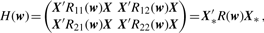
Let 𝒳 be an input matrix, in which each row is an individual and each column is a numerical vector of gene expressions or a categorical vector of SNPs (in genes). Let E be the set of genes for which expressions are measured in 𝒳 and Q be the set of SNPs in 𝒳, indicating that |E|+|Q| is the total number of columns of 𝒳. To test the three-way interaction, we choose one combination, i.e. two genes (e₁ and e₂) and one SNP (q) out of E and Q, respectively, and we write 𝒳(e₁, e₂, q) which has only three columns of 𝒳, corresponding to e₁, e₂ and q [we write 𝒳(e, q) when we choose only one gene e out of E and q out of Q]. Hereafter, until Section 3.6, we assume that we already choose one combination.

For gene expressions, let X=(X₁,…, X_K)′∈ℝ^K be a K-dimensional numerical variable, taking value x=(x₁,…, x_K)′. We note that using two genes in expression does not necessarily mean K=2. For example, for two genes, we can set K=3, where X₁, X₂ and X₃ correspond to one gene, the other gene and the interaction between these two genes, respectively. For genotypes, let C be the number of groups (or classes), and in fact, C=3. We denote three genotypes by G₁, G₂ and G₃, into one of which each individual falls. Let Y be the class variable, taking value y, where Y=(Y₁, Y₂)′∈{0, 1} × {0, 1}. Here, we note that y takes the following values: y=(1, 0)′ if x∈G₁, y=(0, 1)′ if x∈G₂ and y=(0, 0)′ if x∈G₃. We denote N inputs (individuals) by X=(x₁,…, x_N)′ and Y=(y₁,…, y_N)′=(y⁽¹⁾, y⁽²⁾), which can be classified into N₁, N₂ and N₃ inputs for G₁, G₂ and G₃, respectively. The average expression values can be defined for each class c and all classes: and ⁠, respectively, where ⁠. I_K is the identity matrix of size K, and 1 is an n-dimensional vector in which all elements are 1.

We incorporate some basic statistics: and ⁠, where T=B+W. We can further define covariance matrix S_c for class c, and total covariance matrices S and S_T, and ⁠. We note that W = ∑_c=1^CN_cS_c and ⁠.

We show the multivariate normal distribution, having two parameters, μ_c and Σ_c (the mean and the covariance matrix of class c), and the log-density (log-likelihood) function of this distribution can be given as follows:

(1)

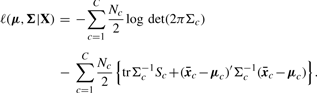
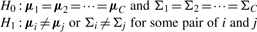
From this equation, we can see that ⁠, covariance matrix S_c and covariance matrix S can be the maximum likelihood estimators of μ_c, Σ_c and Σ (=Σ₁=···=Σ_C), respectively.

We briefly describe likelihood ratio test (LRT), which will be used. We first assume that examples x₁, x₂ ,…, x_n are generated according to parameter vector θ. Let H₀ : θ∈Ω₀ be a null hypothesis and H₁ : θ∈Ω₁ be the alternative hypothesis. The statistic λ for testing H₀ against H₁ can be defined as λ=L₀^*/L₁^*, where L₀^* and L₁^* are the maximum likelihoods under θ∈Ω₀ and θ∈Ω₁, respectively. Usually we can use the log-likelihood ratio (LLR), −2logλ=2(ℓ₁^*−ℓ₀^*), where ℓ₁^*=logL₁^* and ℓ₀^*=log L₀^*. We note that this statistic follows χ_q−r² distribution as N→∞, where q−r is the degree of freedom (df) of the χ² distribution.

3.2 Finding three-way interactions: interaction test (Likelihood Ratio Test of Logistic Regression, LRTLR)

A standard and exact approach for our problem is LRTLR (McCullagh and Nelder, 1989), which we simply call interaction test in this article.

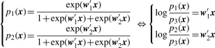
3.2.1 Logistic regression

We first denote the probability that x is in G₁ by p₁(x), and similarly the probability that x is in G₂ by p₂(x), by which the probability that x is in G₃ is p₃(x) (=1−p₁(x)−p₂(x)). We use logistic regression to link these probabilities to K-dimensional input x by using weight parameters (or coefficients) w=(w₁′, w₂′)′, where w₁=(w₁₀, w₁₁,…, w_1(K−1))′, w₂=(w₂₀, w₂₁,…, w_2(K−1))′ as follows:

(2)

Here, we denote p₁(x), p₂(x) and p₃(x) by p₁(x; w), p₂(x; w) and p₃(x; w) (=1−p₁(x; w)−p₂(x; w)), respectively, because they can be functions of w. We can then write the likelihood of logistic regression for given N examples and parameters w, as follows:

where y_i=(y_i1, y_i2)′.

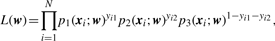
3.2.2 Parameter estimation

We can obtain the maximum likelihood estimator ŵ for w by maximizing the log-likelihood l(w)=log L(w). A standard approach for this purpose is the Newton–Raphson method, which is an iterative gradient descent, having the following updating rule by which we can have ŵ^(t+1) at the (t+1)-th iteration, using ŵ^(t) of the t-th iteration:

(3)

where Hessian matrix H(w) (=∂²l/∂w∂w′) and gradient vector U(w) (=∂l/∂w) can be given in the following:

where X_*=diag(X, X) (block diagonal matrix of X), a(w)=(a₁(w)′, a₂(w)′)′ where a_j(w)=y^(j)−p_j(w) and p_j(w)=(p_j(x₁; w),…, p_j(x_N; w))′ (j=1, 2).

where N × N matrix R_jk(w) (j, k=1, 2) is given by R_jj(w)=diag{p_j(w)⊙(p_j(w)−1)} and R_jk(w)=diag{p_j(w)⊙ p_k(w)} (j≠k).

Finally, the updating rule of the Newton–Raphson method for logistic regression can be rewritten in the following:

(4)

In practise, we start with some initial values ŵ⁽⁰⁾ and update ŵ^(t+1) according to Equation (4) until the following equation is satisfied:

(5)

where δ is set at a certain value.

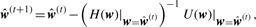
3.2.3 Interaction test

We then examine the significance of the interaction in expression between two genes in terms of classes of another gene. Let x_i1 and x_i2 be expression values of the corresponding two genes for input i. The interaction term is x_i1x_i2, meaning that our purpose is to find the case that the logistic model is well fitted to the data when this term is added. We then let x_i=(1, x_i1, x_i2, x_i1x_i2)′ and w=(w₁₀, w₁₁, w₁₂, w₁₃, w₂₀, w₂₁, w₂₂, w₂₃)′, and the logistic model with the interaction term is given as follows:

If w_c3=0, the model does not have the interaction term, meaning that the null hypothesis and w₀ are given as follows:

(6)

Then the test statistic, LLR and its asymptotic distribution can be given:

(7)

where χ₂²(α_i) is the χ² distribution with the df of two, meaning that interacting genes can be obtained as those which have lower P-values under this distribution than the input significance level α_i. We run interaction test 100 times over four examples in Figure 1, and Table 1 shows the average results over the 100 runs. This table clearly shows that the P-value is very large for Figure 1a–c, while that is zero for Figure 1d, indicating that intraction test can detect our target sample correctly.

Figure 2 shows a pseudocode of interaction test. We can write interaction test by function Interaction_test(e₁, e₂, q, α_i), which outputs one if given example (e₁, e₂, q) has the three-way interaction; otherwise zero. A significant drawback of interaction test is computational inefficiency. In fact, Equation (6) shows K=8, meaning that Newton–Raphson needs to compute an 8 × 8 inverse-matrix at each of its iteration procedure.

Fig. 2.

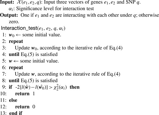
Pseudocode of interaction test.

Open in new tabDownload slide

3.3 Key idea for speeding-up interaction finding

A basic idea for accelerating the finding of a three-way interactions is to prune some combinations, to which interaction test does not have to be applied. From Equation (7), we can see that the interacting genes should have a larger LLR. Figure 3 shows a schematic figure, in which we plot the log-likelihood without the interaction term in the left-hand side and with the interaction term in the right-hand side. We note that the range of the log-likelihood can be limited, because the maximum log-likelihood is zero and the minimum log-likelihood can be given by the case of the uniform distribution for p_i(x). The LLR in question can be then given by the distance being shown by a dotted line in Figure 3. Thus, two interacting genes should have a long dotted line, meaning that the point in the left-hand side should be lower and that in the right-hand side should be higher. This observation indicates that we can prune the following two cases: (I) a large likelihood can be obtained without the interaction term, and (II) only a small likelihood can be obtained even if we use the interaction term. These (I) and (II) correspond to areas I and II, respectively, in Figure 3. We then attempt to efficiently detect examples in areas I and II by assuming the normality on data distribution.

Fig. 3.

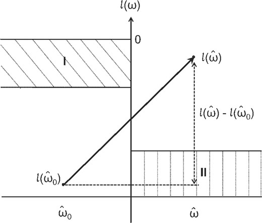
LLR and its components.

Open in new tabDownload slide

3.4 Linear discriminant analysis

Area I in Figure 3 contains examples in which expressions can be easily separated into three classes without the interaction term, as shown in Figure 1b and c. Thus, in this case, we can consider a simpler, easily computable estimation method for parameters of the logistic regression model without the interaction term, and if the likelihood for a given combination by that model is high enough, this combination can be pruned. For the simpler estimation method, we use linear discriminant analysis (LDA), which assumes that x follows the normal distribution N(μ, Σ) with the same covariance Σ for all three classes (Hastie et al., 2001). We skip the detail of this method due to space limitations because in our experiment only a small part of all given examples can be pruned by LDA. Interested readers should refer the Supplementary Material. We can write LDA by function LDA(e₁, e₂, q, α_i) [or LDA(e, q, α_i)], which outputs one if given example (e₁, e₂, q) [or (e, q)] should be pruned; otherwise zero.

3.5 Randomness test

Area II in Figure 3 contains an example for which the maximum likelihood with the interaction term is very low, implying that expression values are almost randomly distributed in terms of classes, as shown in Figure 1a. To detect the randomness of expression values, if we use a faster hypothesis test for randomness than Newton–Raphson, we can speed up the procedure for finding the three-way interaction. We assume that expression values follow the K-dimensional normal distribution for each class of genotypes, and under this assumption, we present our approach, which combines multivariate ANOVA (MANOVA) and Box's M test (Mardia et al., 1979). We can set K=2 for our test, meaning that the largest matrix size is 2 × 2, making the computation very efficient.

3.5.1 MANOVA

MANOVA considers the following null hypotheses over the means:

For testing H₀ against H₁, we use LLR, −2logλ (=2(ℓ₁^*−ℓ₀^*)). By replacing Σ_c in Equation (1) with Σ and using the maximum likelihood estimators and S for μ_k and Σ, respectively, we have the following:

(8)

On the other hand, for the log-likelihood under null hypothesis, we can use the maximum likelihood estimators and S_T for μ_k and Σ, respectively, and we have the following:

(9)

Thus, the statistic can be given as follows: ⁠. We can further see that q is and r is ⁠.

We conducted MANOVA over four samples in Figure 1, and Table 2 shows the resultant average over 100 runs with SDs in parentheses. The P-value of MANOVA for (a) was high (0.53), whereas that for (b) [and (c)] was zero, meaning that MANOVA can discriminate (a) from (b) [and (c)]. However, the P-value of (d) was also high (0.94), meaning that MANOVA could not separate (a) from (d). Thus, we need another hypothesis test, which can distinguish (a) from (d).

3.5.2 Box's M test

We then consider the following hypotheses over the covariance:

Here, ℓ₀^* can be given by ℓ₁^* of MANOVA [i.e. Equation (8)], and ℓ₁^* can be obtained by using maximum likelihood estimators and S_k for μ_k and Σ_k, respectively, in Equation (1).

(10)

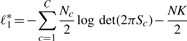
Thus, the statistic is −2logλ=∑_c=1^CN_clog det(S_c⁻¹S). Here, q is and r is ⁠.

We run Box's M test over four samples in Figure 1, and Table 2 shows the results. This result shows that the P-value of (a) was high (0.70), whereas that of (d) was zero, meaning that M-test separated (a) from (d). However, this time, this test could not discriminate (a) from (b) [and (c)], since the P-value of (b) [and (c)] was also high. Thus, this result showed that Box's M test can be a complement of MANOVA, implying that we can combine these two tests for detecting random distributions such as Figure 1a.

3.5.3 MC test (MANOVA + M Test)

We finally consider the following hypotheses over both the means and covariances:

We emphasize that this test suits our purpose the most, although this is an unpopular statistic and not named. We then call this test as MC test. Interestingly, ℓ₀^* of this test is given by ℓ₀^* of MANOVA, i.e. Equation (9) and ℓ₁^* is given by ℓ₁^* of M test, i.e. Equation (10). Thus, the statistic of MC test is given as follows:

(11)

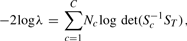
since ⁠. Here, and ⁠, meaning that df is 10 in our case. Figure 4 shows a pseudocode of MC test. We can write MC test by function MC_test(e₁, e₂, q, α_m), having significance level α_m as an input which removes given combination (e₁, e₂, q) if its P-value is larger than α_m, meaning that a larger number of combinations can be removed if α_m is smaller. This function outputs one if (e₁, e₂, q) should be pruned; otherwise zero.

Fig. 4.

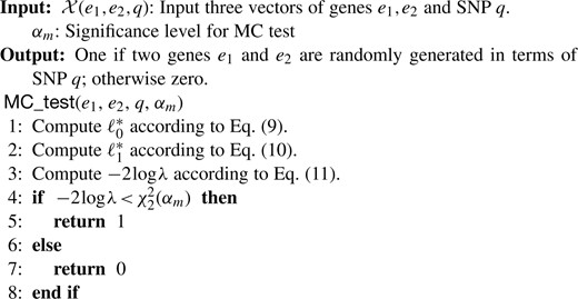
Pseudocode of MC test.

Open in new tabDownload slide

We checked the performance of MC test using synthetic four samples of Figure 1. Table 2 shows that all P-values are zero, except (a) with the P-value of 0.60, indicating that MC test can successfully detect (a) out of the four examples and is expected to work on real data as well.

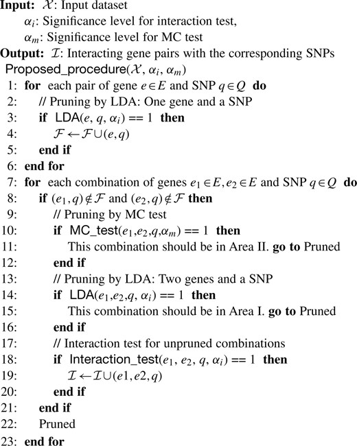
3.6 Proposed procedure

Figure 5 shows a pseudocode of our entire procedure. We can first check each pair of a gene and a SNP by LDA, and if the log-likelihood is high, this pair is stored to be pruned. We then generate all possible combinations of two genes and a SNP out of given data. For each of these combinations, it is first pruned if it contains the stored gene–SNP pair. Then, LDA and MC test are run in sequence for pruning, and finally interaction test is applied to the remaining. Hereafter, we call our proposed procedure FTGI, standing for Fast finding Three-way Gene Interactions, whereas we call the approach of running Interaction Test Only over all possible combinations as ITO. More details of our proposed method is shown in the Supplementary Material.

Fig. 5.

Pseudocode of our entire procedure: FTGI.

Open in new tabDownload slide

4 EXPERIMENTS

4.1 Data

We used the human brain-derived dataset of Myers et al. (2007), which originally has 193 rows (individuals) and 14 078 numerical columns (corresponding to gene expressions) and 366 140 categorical columns (corresponding to SNPs). We first removed the columns containing missing values and the columns which have a genotype to which only less than 10 individuals are assigned. Our purpose is to find three-way gene interactions, and so we further removed SNPs which are neither in coding regions nor in introns, by specifying genes on sequences using the FTP site of NCBI Mapviewer for Homo sapiens. Finally, we obtained 5269 numerical vectors (in expression of genes) and 13 411 categorical vectors (in genotypes of SNPs) for 193 individuals, which we call the Source dataset. Myers et al. (2007) collected the original dataset from human brains, and so we focused on neurodegenerative diseases [including Alzheimer's disease (AD) and Parkinson's disease, etc.] out of five disease pathways in the KEGG disease database (Kanehisa et al., 2008), resulting in 142 genes which we call Neuro. All experiments were run on a machine with Dual-Core AMD Opteron 2222 SE (3.0 GHz) and 18 GB RAM. Throughout Section 4, each P-value is shown by log₁₀(P-value).

4.2 Results and discussion

4.2.1 Speeding-up finding three-way interactions and pruning accuracy

We examined the improvement in time efficiency by FTGI over ITO. Figure 6 shows the real computation time of ITO and FTGI, when we changed the number of combinations randomly chosen from the source dataset. We here focused on Area II of Figure 3 only, since we found that in the Source dataset of Area I had only a small number of examples, which do not affect the efficiency greatly. This figure clearly shows that as α_m decreased, the amount of running time of FTGI became smaller for any size of inputs, by pruning a larger number of them. In particular, at α_m of 0.001, FTGI runs approximately 10 times faster than ITO, resulting in only ∼2 h for 10⁷ combinations, being a sizable improvement. This means that for 5 × 10¹⁰ (= 50 000 SNPs × 1000 genes × 1000 genes) combinations, FTGI just needs only a couple of days with 100 CPUs, while ITO needs more than a month.

Fig. 6.

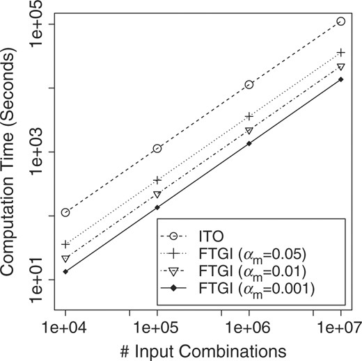
Computation time improvement by reducing α_m.

Open in new tabDownload slide

The α_m controls the number of pruned combinations, and Table 3 shows the pruning rate, i.e. the ratio of pruned combinations to all input combinations, with varying α_m for 10⁷ input combinations. We further checked the pruning accuracy, which can be defined as the overlap between the resultant top 𝒦 (set at 100) combinations by P-values of ITO and those of FTGI. Table 3 shows that for α_m of 0.05, FTGI can prune around ∼70% of input combinations with pruning accuracy of almost 100%. If α_m is reduced to 0.001, ∼94% inputs can be pruned, keeping the pruning accuracy of ∼85%. This high pruning rate effects the time efficiency of FTGI.

We note that all results in this section were averaged over three runs at each corresponding setting.

4.2.2 Detecting three-way interactions

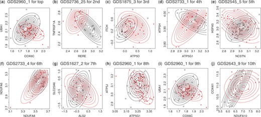
We then generated all combinations from the Source dataset, focusing on the genes in Neuro, meaning that we had totally ∼3 × 10⁸ combinations (= 13 411 SNPs × 142 genes × 142 genes). We then run FTGI with α_m of 0.001 over these combinations. Figure 7 shows the gene expressions of the resultant top 10 combinations in terms of P-values. We note that these P-values of interaction test were computed by the procedure in Section 3.2. Each of Figure 7 is a 2D diagram on which expression values of the corresponding two genes are plotted with Contour lines for each genotype. This figure shows that the topographical distribution of different genotypes are clearly crossed in all cases, meaning that in each of all the top 10 combinations, genes are interacting in expression, being controlled by genotypes, as shown in Figure 1d.

Fig. 7.

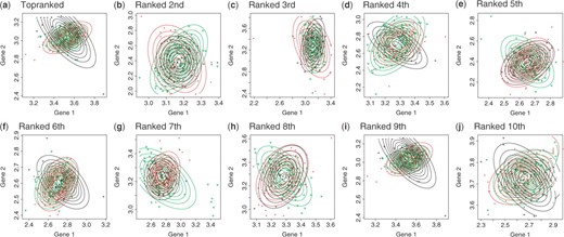
Expressions of two genes under three genotypes of another gene for top 10 (a–j) ranked three-way interactions out of 3 × 10⁸ combinations.

Open in new tabDownload slide

Table 4 shows the detail (Gene name for one SNP and the name with GeneID, the definition and the pathway for each of two interacting genes in expression) of the 10 three-way interactions in Figure 7, all information in this table being retrieved from KEGG.² For example, the first interaction of Table 4 shows the switching mechanism of two genes, COX6C and UBA1, being controlled by a SNP in LARP4.

4.2.3 Validating detected interactions with permutations

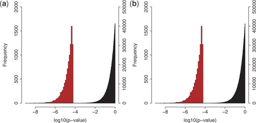
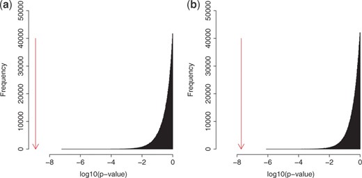
To confirm the statistical significance of the detected three-way interactions, we conducted permutations by measuring P-values of ‘null data’, generated in the following three manners, and comparing them with those of the interactions we detected. We first show the results of permutation tests when we use Null data 1 and 2. Figure 8 shows the distribution of P-values of null examples, being located in the right side, for Null data 1 and 2. In this figure, the distribution of P-values for the top 10 000 interactions detected by FTGI is located in the left side. This figure shows that the red-colored distribution is clearly separated from the black-colored one, meaning that the detected three-way interactions have significantly small P-values. For Null data 3, we show the result, focusing on two cases (the top and the 10th interactions), since the trend of results was kept the same for all 10 interactions in Table 4. Figure 9 shows the distribution of P-values of null examples generated from the top interaction (or the 10th), with the P-value of the top (or the 10th) interaction by an arrow. This figure indicates that the P-value of the top (or the 10th) interaction is clearly distant from the P-value distribution of null examples, implying that P-values of the detected interactions are statistically significant.

• Null data 1: we randomly chose 10 000 combinations out of all combinations using the Source dataset (13 411 SNPs × 5269 genes × 5269 genes) and randomly permuted the genotypes of these combinations 100 times. Totally, we had one million null examples.

• Null data 2: we randomly chose 10 000 combinations out of all combinations using the Neuro dataset (13 411 SNPs × 142 genes × 142 genes) and randomly permuted the genotypes of these combinations 100 times. Totally, we had one million null examples.

• Null data 3: we permuted the genotypes of each of the detected top 10 interactions in Figure 7 one million times, resulting in one million null examples for each combination.

Fig. 8.

Distributions (left side) of P-values of the top 10 000 interactions detected by FTGI, with those (right side) of Null data (a) 1 and (b) 2.

Open in new tabDownload slide

Fig. 9.

The P-values of the (a) top and (b) 10th interactions (shown by arrows) and the distributions of P-values of the corresponding null examples generated.

Open in new tabDownload slide

4.2.4 Validating detected interactions with GEO

To confirm the reliability of the interactions in Table 4, we tried to find, for each gene pair, the switching mechanism in expression which can be controlled by some experimental condition of gene expression. This is because if found, this directly means that the corresponding gene pair can be controlled by another categorical factor, such as genotypes of another gene.

For this purpose, we used GEO (version of June 1, 2009; Barrett et al., 2007), from which we found 2089 GDSs (gene datasets) which are annotated. Out of the 2089 datasets, we selected datasets which satisfy all the following four conditions for each gene pair in Table 4: (i) expression values of the corresponding gene pair are contained; (ii) the total number of experiments is ≥50; (iii) experimental conditions can be divided into two or more classes; and (iv) each class has 10 or more experiments. We then obtained 36 datasets.³ For each gene pair of the top 10 list, we conducted interaction test by using pairwise (binary) classes in each dataset and ranked them according to P-values of interaction test. Table 5 shows a list of datasets, each giving the lowest P-value for each gene pair of the 10 interactions in Table 4. For example, for COX6C and UBA1, the gene pair of the first interaction of Table 4, we found a switching mechanism in GDS2960_1 with the P-value of −3.9532, showing the statistical significance of this mechanism. This directly indicates that there must exist a switching mechanism in expression between these two genes under the alteration of experimental conditions which is specified by the annotation of GDS2960_1. In fact, Table 5 indicates that the switching mechanism happens between patients of Marfan syndrome and controls. This type of explanation is possible for all 10 GDSs in Table 5 by using annotations in this table. As well all P-values shown in Table 5 are small enough,⁴ supporting the reliability of the three-way interactions in Table 4 which our method detected. Furthermore, Figure 10 shows the real expression values of two genes, being categorized into two classes, for each GDS of Table 5. These orthogonal Contour plots also assist the reliability of three-way interactions that we detected in Table 4.

Fig. 10.

(a–j) Expressions of two genes which give the smallest P-value of interaction test in the corresponding GDS of GEO.

Open in new tabDownload slide

We further briefly checked the genes having SNPs in the first and the third interactions in Table 4: (i) the first interaction in Table 4 has two genes, COX6C and UBA1, which is controlled by a SNP in LARP4, i.e. La ribonucleoprotein domain family member 4. This gene was already known as an important gene in both AD and aging, being already pointed out that LARP4 increases expression with increasing AD progression and normal aging (Miller et al., 2008). As our focus was on 142 genes on neurodegenerative diseases including AD, the known function on LAPR4 is consistent enough with the interaction with COX6C and UBA1, being possibly in the switching mechanism. (ii) The gene with the SNP in the second interactions in Table 4 was a hypothetical one, but the third interaction has two genes, ATP5D and ITCH, being controlled by a SNP in RPS3AP5, which is a pseudogene of RPS3A, i.e. ribosomal protein S3A. This gene is known to be downregulated in the same manner as some genes in oxidative phosphorylation pathway (Welle et al., 2003), which includes ATP5D. Thus, these observations reveal the possibility that the third interaction also may exist as the switching mechanism in expression of two genes, i.e. ATP5D and ITCH.

Overall our extensive analysis has implied that the detected three-way interactions can exist. These results show the potential of our approach to explicate complex biological systems appearing in modern biology and medical sciences.

5 CONCLUDING REMARKS

We have presented a fast method for finding three-way gene interactions from transcript-and genotype-data and showed experimental results obtained by applying this method to ∼3 × 10⁸ human brain samples. In our experiments, we confirmed the three-way interactions that we found in various manners. Possible future work would be to apply our approach to various types of transcript- and genotype-data further to uncover three-way gene interactions, i.e. biological switches by genotypes.

ACKNOWLEDGEMENTS

The authors would like to thank anonymous reviewers for their helpful comments and advice.

Funding: Grant-in-Aid for Young Scientists 20700134, 20700269, 21680025 from Ministry of Education, Culture, Sports, Science and Technology (MEXT, in parts); the Functional RNA Project of New Energy and Industrial Technology Development Organization (NEDO, in parts).

Conflict of Interest: none declared.

REFERENCES

Author notes