Statistical lower bounds on protein copy number from fluorescence expression images Open Access

Abstract

1 INTRODUCTION

Fluorescent imaging is widespread in the analysis of mRNA and protein expression in single cells, in populations of cells and within tissues or organisms. Such data are useful for a wide variety of purposes: determining the effects of gene knockouts, over/underexpression, or promoter manipulations, understanding regulatory networks, determining co-expression of genes or co-location of gene products, which may indicate complexing, identifying markers for tissue types or processes, inferring protein function and so on.

As useful as such data are, a limitation is that it usually only gives relative expression values. Greater fluorescent intensity implies greater expression, but the actual concentrations or copy numbers of molecules being imaged are usually not known. Knowing expression in absolute terms can be important for detailed quantitative modeling (Brown and Sethna, 2003) and for extracting biologically meaningful parameters. For example, most current fitting methods, even if couched in chemical terms, express reaction rates in fluorescence units (e.g. Tian et al., 2007), rather than in molecules or moles. Absolute expression is also relevant for understanding the sources of noise or variability in gene expression (Bar-Even et al., 2006; Bundschuh et al., 2003; Rao et al., 2002; Raser and O'Shea, 2005; Rosenfeld et al., 2005; Swain, 2004; Swain et al., 2002; Thattai and van Oudenaarden, 2001; Vilar et al., 2002) and potentially for recent analyses of information processing in gene regulatory networks (Andrews and Iglesias, 2007; Andrews et al., 2006; Gregor et al., 2007; Libby et al., 2007; Tkacik et al., 2008).

There are imaging techniques that can result in concentration or copy number information, such as fluorescence- and image-correlation spectroscopy (Elson and Magde, 1974; Wiseman et al., 2000), fluorescence-intensity distribution analysis (Kask et al., 1999) and photon-counting histogram analysis (Chen et al., 1999). Alternatively, the intensity signal can be calibrated by measuring expression of mRNAs or proteins that are at known concentrations (e.g. Bar-Even et al., 2006; Gregor et al., 2007). However, none of these approaches is nearly as common in practice as direct, uncalibrated measurement of fluorescent intensity.

We present two different methods for estimating copy numbers of fluorescently labeled molecules from single uncalibrated images. We were particularly motivated by our previous work on modeling regulation of genes in the segmentation network of Drosophila melanogaster (Perkins et al., 2006), and we use data on this system in our study. However, our approach is readily applicable to similar data from other organisms. Both methods rely on variability in the expression data to estimate absolute expression. The key intuition is that variability is greater when absolute expression is smaller, because the inherent stochasticity of the biochemistry is more pronounced when molecule numbers are small. However, as we work with single still images, it is variation between cells (or more properly, between nuclei) that we exploit, rather than variability over time. This type of variability has previously been exploited to estimate protein concentration in growing colonies of Escherichia coli (Rosenfeld et al., 2005, 2006). One of our methods is very similar to one of the approaches used in these works.

2 BIOLOGICAL SYSTEM AND DATA

Within several hours after fertilization, one of the first developmental gene networks to come online in the Drosophila embryo is the segmentation network (Rivera-Pomar and Jäckle, 1996; Scott and Carroll, 1987). The segmentation network establishes patterns of gene expression that mark the eventual body segments of the grown organism—divisions of the body along the anterior–posterior axis. The network is broadly organized as a genetic cascade, with successive groups of genes (maternal, gap, pair-rule, segment polarity) expressing ever more spatially refined signals (Fig. 1A).

Fig. 1.

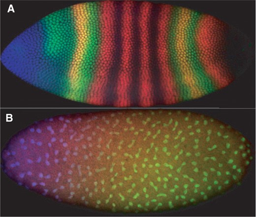
(A) An image from FlyEx (Poustelnikova et al., 2004) showing expression of maternal-class gene bicoid (blue), gap gene giant (green) and pair-rule gene even-skipped (red) in Drosophila embryo as9. (B) An image showing an embryo (ab18) in which nuclei have just divided or are finishing dividing, and in which sibling pairs can readily be identified.

Open in new tabDownload slide

The data that we use are available online from the FlyEx database (Poustelnikova et al., 2004), which contains images of Drosophila embryos undergoing segmentation. The experiments measured gene expression using fluorescence tagged antibodies in fixed embryos. Specifically, primary antibodies were raised against the segmentation genes by repeated injection into either rabbits, guinea pigs or rats (Janssens et al., 2005; Kosman et al., 1998). The fixed embryos were incubated with dilutions of these antibodies. The embryos were also incubated with commercially available secondary antibodies that bind to the primary antibodies, and that are cross-linked to fluorescent dyes (Alexa488, Alexa555 and Alexa647). These dyes were excited by means of lasers, and imaged using a confocal microscope. For each embryo, a 1024 × 1024 pixel image was captured, with each of the three channels in the image recording the intensity of a different tagged protein.

At this stage of development, the embryo is a syncytium—a single cell with multiple nuclei that divide periodically and roughly simultaneously. The proteins represented in the database are all transcription factors and they tend to congregate in the nuclei. Thus, the nuclei can readily be identified. A series of image processing algorithms locates the nuclei and calculates the expression of each protein in each nucleus in terms of intensity units, ranging from 0 to 255 (Janssens et al., 2005; Surkova et al., 2009). It is this per-nucleus-derived data, also available from the FlyEx database, to which our methods are applied.

3 METHODS

Our methods for estimating protein copy number assume that the observed intensity of a nucleus in a particular channel is proportional to the copy number of the corresponding protein in that nucleus. The proportionality factor, denoted ν, may vary for different proteins, but is assumed to be consistent across different embryos imaged in the same manner. Both methods work by estimating ν, from which protein copy numbers in each nucleus can be derived based on their intensity. The two methods are not alternatives to each other, but rather apply in different situations.

We describe the methods as producing statistical lower bounds on protein copy number. ‘Statistical’ comes from the fact that the methods posit probabilistic models about how the intensity data are generated. The ‘lower bound’ comes from the fact that the models attribute all variability in protein expression to fundamental stochastic chemical processes. In fact, the data include other sources of variability, or noise, which we discuss further below. As such, the true variability in protein expression tends to be overestimated by our methods, resulting in copy number estimates that are biased low.

3.1 Binomial estimation method

The binomial estimation method applies to embryos in which nuclei have recently undergone division, and sibling pairs can be easily identified (Fig. 1B). The method assumes that proteins in the mother of each sibling pair pass independently and with equal probability to each daughter nucleus. The difference in intensities of the siblings can then be related to absolute concentration.

More formally, let i1 and i2 denote the members of a sibling pair, and i denote their (unobserved) mother nucleus. Let N_i be the unknown number of fluorescent molecules in the mother, and N_i1 and N_i2 the unknown numbers of molecules in the daughters. We assume that N_i1 and N_i2 are both distributed as binomial with N_i tries and p = 1/2 success probability. Of course, N_i1 and N_i2 are not independent binomial random variables. Assume that no protein is lost in the division process, then N_i1 + N_i2 = N_i. One justification for this model is as follows. Many of the transcription factor molecules under discussion bind the DNA non-specifically in ‘random’ places. Before the nuclear division, each protein can thus be thought of as equally likely to be on the DNA copy that goes to one daughter as it is to be on the DNA copy that goes to the other daughter. Proteins that are not bound to the DNA, assuming they are uniformly distributed throughout the nucleoplasm, are also equally likely to end up in either daughter nucleus. This is because each daughter receives close to half of the nucleoplasm of the mother.

We assume that the observed fluorescence is proportional to the number of molecules present: O_ij=νN_ij. If we can estimate ν, then we can estimate protein copy number in each nucleus simply by solving the previous equation for N_ij. Each sibling pair provides us with one estimate for ν as:

(1)

This is very similar to the estimator used by Rosenfeld and colleagues (2005, 2006), who applied it to sibling data from fluorescent image sequences of growing colonies of E.coli. The main difference is that Rosenfeld et al., working with time series data, also had intensity measurements for the mother cells before division, and these could be used in place of the denominator above. One mathematical rationale behind the estimator is that its expected value, treating N_i as given and N_i1, N_i2, O_i1 and O_i2 as dependent random variables, is:

The estimates from each sibling pair can be combined into an overall estimate for ν based on simple averaging: ⁠, where M is the total number of sibling pairs. This estimator can also be justified as giving the value of ν that maximizes the likelihood of the O_ij, if one approximates the binomial distributions with normal distributions having the same means and variances. (Proof omitted.) Rosenfeld et al. (2006) also explored models with observation noise, and derived a Bayesian parameter estimation approach. We return to this issue in Section 5. The crux of the matter, however, is that simple noise models are not consistent with the variability we see in the data or our estimators, and so we have not attempted any correction.

To apply this method to a given image, one must identify the sibling pairs. For our study, we identified 22 embryos in the FlyEx database that showed a reasonable number of pairable nuclei. We identified these embryos by visual examination of the fluorescence images of all cleavage cycle 10 through 13 embryos, as well as cleavage cycle 14A, time class 1 embryos—a total of approximately 400 embryos. We experimented with several algorithms to automatically pair nuclei, primarily based on proximity. However, given the relatively small number of images to be analyzed in this way and desiring to have the highest fidelity pairings possible, we ultimately settled on pairing the nuclei by hand (aided by an interactive MATLAB routine we developed). We did not pair up all nuclei in each image, as appropriate pairings were not always clear. We also avoided pairing nuclei near the edge of the embryo, as the intensity of these nuclei was often affected by their proximity to the edge. The on-line material contains a complete specification of the pairings used. We leave reliable automatic pairing as a topic for future research.

3.2 Poisson estimation method

Our second approach is intended for embryos that are significantly past their most recent nuclear division, and are at a more steady- state behavior. As with the binomial estimator, the essential intuition is that variability in expression can somehow be related to copy numbers. However, it is far from clear what an appropriate model for the steady-state distribution of protein copy number might be. In simpler, prokaryotic situations, stochastic chemical kinetic models have been quite successful at capturing and explaining stochasticity in gene expression (see Raj and van Oudenaarden, 2008, for a recent review). Such models usually incorporate stochastic production and decay of mRNAs and proteins, and possibly other processes. A common finding is that variability in protein levels is often due more to variability in the mRNA levels than to the inherent stochasticity in protein production and decay. Bar-Even et al. (2006), in an empirical study using Saccharomyces cerevisiae, found that under a variety of conditions and for a variety of genes, variance in protein expression across cells in a population was proportional to mean protein expression. By analyzing different possible sources of expression variability, they came to the conclusion that mRNA fluctuations were the main cause, just as in the bacterial models. On the other hand, Bagh et al. (2008), analyzing expression driven by plasmids in E.coli, observed that the SD of expression scales with mean expression, with most variability attributable to cell size.

3.2.1 Model assumptions and estimator

As in Bar-Even et al. (2006), we find that protein expression variance scales roughly linearly with mean protein expression (Fig. 2). However, we consider it unlikely that mRNA fluctuations are as significant a source of noise as they are in that study or in the bacterial models. The Drosophila embryo is not cellularized at this stage. For most of the segmentation genes, mRNAs are transcribed and exported from the nuclei and accumulate in inter-nuclear space, apparently at much greater concentration than is typical for the models or experiments cited above. This observation is based on mRNA stains in embryos at the same developmental stage (Jaeger et al., 2007), although like proteins, mRNA copy numbers have not been quantified in this setting. Proteins are translated from mRNAs in the extra-nuclear space, and are taken up quickly by nearby nuclei, where they may eventually decay. Assuming that the total amount of mRNA in the vicinity of a nucleus is relatively constant, the main factors influencing protein expression would thus be a stochastic production and uptake along with stochastic decay.

Fig. 2.

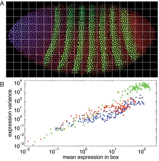
The relationship between mean and variance of protein expression. (A) An embryo image (bd5) divided into a grid, with 20 divisions along the anterior–posterior axis and 10 divisions along the dorsal–ventral axis. For the blue and red channels (representing Bicoid and Caudal protein, respectively), expression is relatively constant within each grid box. This is less true for the green channel (representing Even-skipped protein). (B) For each box we compute the mean and variance of the per-nucleus expression values for all nuclei within the box. If expression variance scales with mean, as observed by Bar-Even et al. (2006) for S.cerevisiae, then we should see a linear relationship between log variance and log mean, with a slope of approximately one. This is consistent with the data from this embryo. Best fit lines have slopes of 1.06 (blue channel), 0.94 (red channel) and 1.73 (green channel). The larger slope for Even-Skipped likely results from the spatially non-uniform expression pattern within each grid cell, adding another source of variance to the data besides real biological variability, rather than a true violation of the proportionality of mean expression and the variance of expression. Similar results were obtained from other embryos.

Open in new tabDownload slide

Based on this reasoning, and consistent with the observation in Figure 2, we assume that the number of proteins in a nucleus, N_i, is Poisson distributed, with a nucleus-specific Poisson parameter λ_i. As for the previous estimator, we assume that the observed fluorescent intensity of a nucleus, O_i, is proportional to the expression. Thus, O_i=νN_i. Under these conditions,

(2)

If we could estimate the mean and variance of O_i, we could get an estimate of ν, and by extension, an estimate of N_i. The problem is that expression in each nucleus is being driven at a different rate λ_i. With a single observation, O_i, of each nucleus, how can we estimate both the first and second moments?

The solution we propose is to rely on the spatial smoothness of the nuclear expression levels. Nearby nuclei usually show similar expression levels, because they are subject to similar regulatory signals. For each nucleus i, then, we can use other nuclei in the vicinity to estimate E(O_i). Our method for making this estimate is described below. For the moment, assume we have estimates Ê(O_i) for every nucleus. We then produce per-nucleus estimates of ν.

(3)

These estimates are averaged across nuclei, to generate our overall estimate ⁠. This estimator can also be justified as the maximum likelihood solution, if one approximates the Poisson distributions by corresponding normal distributions with the same means and variances. We omit the proof, which is straightforward.

3.2.2 Estimating expected intensity

We propose a local regression scheme to predict the expected intensity of each nucleus. The maternal and gap genes have fairly simple, spatially smooth expression patterns. For these, we generate Ê(O_i) in three steps: (i) find the 20 nuclei closest to nucleus i; (ii) fit their observed intensities by quadratic least squares regression, as a function of anterior–posterior and dorsal–ventral position; and (iii) evaluate the regressor at the coordinates of nucleus i.

For the pair-rule genes, this scheme works to a degree, but can be improved. The expression patterns of these genes have sharp discontinuities and are spatially complex, being present in seven vertical stripes (Fig. 1A). For a nucleus i in one of these stripes, the nuclei that are dorsal or ventral of i and within the same stripe are better predictors of O_i than are nuclei to the anterior or posterior. Finding such nuclei reliably takes some effort, however, as the stripes are not perfectly vertical, but rather are slanted and curved. (‘Splayed’ is the term used in the Drosophila community.) Thus, we begin by applying a coordinate transformation intended to make the stripes vertical. We use a simplified version of a method developed by Spirov and colleagues (Spirov and Holloway, 2003; Spirov et al., 2001, 2002, Fig. 3). Dorsal–ventral coordinates of each nucleus, DV_i, are left unchanged, but anterior–posterior coordinates are transformed as

where s, a and b parameters, and coordinates are expressed as fractions of embryo length. All three parameters are optimized numerically over the discrete set of values {0, 0.025, 0.05,…, 1.5}, to maximize the variance of expression intensity along the anterior–posterior axis. After correcting for splay, we use the same local quadratic regression scheme described above to predict Ê(O_i), except that nearby nuclei are determined based on a weighted Euclidean distance with anterior–postetior distance counting three times as much as dorsal–ventral distance. In this way, ‘nearby’ nuclei are preferentially located dorsal or ventral to nucleus i, which, because of splay correction means within the same stripe. Using a 10% subset of the data, we estimate that the combination of splay correction and preferential dorsal–ventral distance weighting reduces squared prediction error for pair-rule nuclear expression by approximately one-third.

Fig. 3.

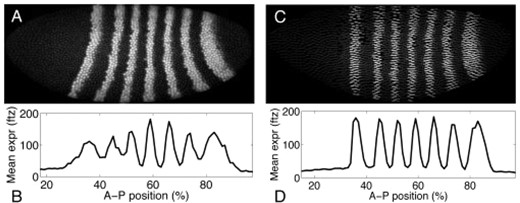
Splay correction for local regression/smoothing of pair-rule gene expression patterns. (A) Red channel of image of embryo FEScc01 (fushi-tarazu gene). (B) Mean intensity as a function of anterior–posterior position. (C) Simulated embryo image after splay correction. (D) Mean intensity after correction. Parameters of the coordinate transform are chosen to maximize the variance, along the anterior–posterior axis, of mean intensity.

Open in new tabDownload slide

4 RESULTS

We applied the binomial method to the hand-pairings for the 22 embryos we identified from our survey of the FlyEx database, and we applied the Poisson method to all cleavage cycle 14A, time class 8 embryos in the database—a total of 130 embryos. For each gene and each method, the estimates for ν are based on the per-nucleus or per-nucleus-pair estimates pooled across all embryos involving that gene. It turned out that taking the simple mean of these individual estimates, as described in Section 3, was problematic. Some of the per-nucleus estimates from the Poisson method were negative—resulting from poor (technically impossible) negative estimates of expected intensity. The binomial and Poisson methods also produced some dramatically large per-nucleus or per-nucleus-pair estimates. When traced back, these obvious outliers had a variety of causes. Some were due to problems with the underlying data, such as falsely detected nuclei in the images or segmentation errors. Some also resulted from poor expected intensity estimates in the Poisson method, particularly for complex parts of the pair-rule expression patterns. As a general hedge against such errors, we used trimmed means to estimate ν, throwing out the 10% largest per-nucleus or per-nucleus-pair estimates before averaging.

Table 1 summarizes the results of the binomial and Poisson estimators. The estimates for ν are shown for each gene, along with the predicted copy number under conditions of maximal expression. The prediction is obtained simply as ⁠, as 255 is the maximum possible intensity in the images. The genes are segregated into three classes according to the standard categories of maternal, gap and pair-rule genes.

Table 1.

Open in new tab

Copy number estimates from the binomial and Poisson estimation methods, along with estimates for the intensity-to-copy-number scale factor ν

.	Binomial method .		Poisson method .
Gene .	.	Peak Copy # .	.	Peak Copy # .
bicoid	0.17	1500	0.35	730
caudal	0.25	1000	0.28	900
giant	0.041	6200	0.15	1700
hunchback	0.19	1300	0.31	820
Krüppel	0.032	8000	0.094	2700
knirps	–	–	0.13	2000
tailless	–	–	0.37	700
even-skipped	0.16	1600	0.98	260
fushi-tarazu	–	–	0.79	320
hairy	–	–	0.78	330
odd-skipped	–	–	0.57	450
paired	–	–	0.87	300
runt	–	–	0.51	500
sloppy-paired	–	–	1.9	140

.	Binomial method .		Poisson method .
Gene .	.	Peak Copy # .	.	Peak Copy # .
bicoid	0.17	1500	0.35	730
caudal	0.25	1000	0.28	900
giant	0.041	6200	0.15	1700
hunchback	0.19	1300	0.31	820
Krüppel	0.032	8000	0.094	2700
knirps	–	–	0.13	2000
tailless	–	–	0.37	700
even-skipped	0.16	1600	0.98	260
fushi-tarazu	–	–	0.79	320
hairy	–	–	0.78	330
odd-skipped	–	–	0.57	450
paired	–	–	0.87	300
runt	–	–	0.51	500
sloppy-paired	–	–	1.9	140

Table 1.

Open in new tab

Copy number estimates from the binomial and Poisson estimation methods, along with estimates for the intensity-to-copy-number scale factor ν

.	Binomial method .		Poisson method .
Gene .	.	Peak Copy # .	.	Peak Copy # .
bicoid	0.17	1500	0.35	730
caudal	0.25	1000	0.28	900
giant	0.041	6200	0.15	1700
hunchback	0.19	1300	0.31	820
Krüppel	0.032	8000	0.094	2700
knirps	–	–	0.13	2000
tailless	–	–	0.37	700
even-skipped	0.16	1600	0.98	260
fushi-tarazu	–	–	0.79	320
hairy	–	–	0.78	330
odd-skipped	–	–	0.57	450
paired	–	–	0.87	300
runt	–	–	0.51	500
sloppy-paired	–	–	1.9	140

.	Binomial method .		Poisson method .
Gene .	.	Peak Copy # .	.	Peak Copy # .
bicoid	0.17	1500	0.35	730
caudal	0.25	1000	0.28	900
giant	0.041	6200	0.15	1700
hunchback	0.19	1300	0.31	820
Krüppel	0.032	8000	0.094	2700
knirps	–	–	0.13	2000
tailless	–	–	0.37	700
even-skipped	0.16	1600	0.98	260
fushi-tarazu	–	–	0.79	320
hairy	–	–	0.78	330
odd-skipped	–	–	0.57	450
paired	–	–	0.87	300
runt	–	–	0.51	500
sloppy-paired	–	–	1.9	140

For the maternal and gap genes, the Binomial and Poisson methods were in broad agreement. For all genes, the estimates of ν by each method were within a factor of four of each other. There was particularly good agreement for the caudal gene. Estimated copy numbers for the proteins corresponding to these genes ranged from the high hundreds to the low-to−mid thousands. The binomial method reported uniformly lower estimates for ν than the Poisson method, and thus predicts higher copy numbers.

The agreement between the two methods was worse for the even-skipped gene, with the binomial estimate for ν being one-sixth as large as the Poisson estimate. The Poisson estimates for ν for the pair-rule genes were mostly in the range of 0.5 to 1.0, making for copy number estimates in the low hundreds of proteins per nucleus.

5 DISCUSSION

Agreement of the binomial and Poisson estimators on the maternal and gap genes is encouraging, giving us some confidence in the methods. However, both methods are expected to produce copy number estimates that are biased low. Their agreement should not be interpreted as evidence of correctness of the estimates. Gregor et al. (2007) performed experiments to calibrate observed fluorescence to absolute expression of Bicoid protein. They estimated that in the highest expressing nuclei, Bicoid is present at a concentration of 55±3 nM, or 33±1.8 molecules/μm³. If we assume that nuclei are spherical with an estimated 6.5 nm diameter, or a volume of 144 μm³, then the Bicoid concentration estimate corresponds to 4750±260 molecules per nucleus. This value is just over three times as large as we obtained from the binomial method, and 6.5 times as large as from the Poisson method. Of course, the Gregor et al. estimate is itself subject to a number of potential biases, and should not be treated as ground truth. To our knowledge, however, it is the only available experimental estimate of Bicoid protein copy number, and it suggests that our estimates may be significantly low. Whether our estimates for other genes are off by a similar factor is unknown.

Wu et al. (2007) used an approach similar in broad strokes to ours to estimate Bicoid protein copy numbers. Bicoid is unique among the proteins studied here in that the protein is translated only at the anterior pole of the embryo, from where it diffuses through the embryo and enters nuclei to regulate transcription. Although this mechanism is much different than that of the other segmentation genes, Wu et al. (2007) show that it too leads to a theoretical expectation of Poisson-distributed copy numbers in each nucleus. They compared fluctuations in computer simulations of stochastic diffusion with observed fluctuations in fluorescent intensity [in data from the FlyEx database (Poustelnikova et al., 2004), though they used different embryos than we did]. From this, they estimated copy numbers in the anterior fifth of the embryo, where the nuclei with the highest expression are, at between 200 molecules per nucleus and 2000 molecules per nucleus, depending on the embryos analyzed. These figures, especially the upper end of the range, are broadly consistent with our estimates for Bicoid. However, this agreement must be viewed with a grain of salt, as both studies are based on data from the same laboratory, and thus may fall prey to similar biases in data collection or processing.

For pair-rule genes, we have no corroborating data and can compare the binomial and Poisson methods only on the even-skipped gene. On that gene, the binomial estimator suggests protein copy numbers six times as large as the Poisson estimator suggests—in the low thousands of proteins per nucleus at peak expression. We suspect the binomial estimator is closer to the truth. One reason is purely mathematical. Both methods are expected to underestimate true copy numbers, but by different and unknown amounts. If both are underestimates, then whichever is higher is closer to being right. Another reason is that the Poisson estimator clearly had difficulty with the spatially fine pair-rule patterns, despite our extra efforts in fitting these patterns. In some parts of the embryos, expression does not vary smoothly as a function of position. For example, Figure 4A shows a close up of an embryo in which nuclei with near-maximal expression of even-skipped are adjacent to nuclei with near-minimal expression of the same. That said, in some cases the Poisson estimator was responding to genuinely greater variability in expression than is seen for the maternal or gap genes. For example, Figure 4B shows a close up of part of an embryo in which expression within the first even-skipped stripe is quite irregular.

Fig. 4.

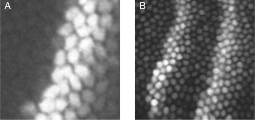
Close-up views of two embryos. (A) Embryo ba3, showing spatial discontinuity in expression of even-skipped, which is fully off in some nuclei and fully on in some adjacent nuclei. (B) Embryo FEScc34, showing significant variability of expression of even-skipped, even within a single stripe.

Open in new tabDownload slide

One motivation for the Poisson estimator is that it is the simplest identifiable model consistent with our observation that variance in expression seems to scale with mean expression. Bar-Even et al. (2006), working in S.cerevisiae, also observed expression variance scaling with the mean. However, they ruled out a Poissonian distribution of protein copy number, because they found variance to be equal to roughly 1000 times the mean of expression, over a wide range of conditions. For a Poisson distribution, the variance is equal to the mean. The same constant of proportionality could not hold in the Drosophila context. If it did, it would imply that our estimates of ν are roughly 1000 times too large, and our copy number estimates are 1000 times too small—that is, true copy numbers in the nuclei of the embryo are in the hundreds of thousands or millions. Nevertheless, it is possible that copy numbers are not Poissionian. Rather they may follow some other distribution for which variance is proportional to the mean, but with a constant of proportionality somewhere between 1 and 1000. Further calibration experiments could resolve this conundrum.

The models above fail to account for many potential sources of noise. This includes noise in the biological system, such as mRNA fluctuations in space or time, diffusion of mRNA or protein, fluctuations in regulatory factors or fluctuations in ribosomes. The models also do not account for imaging or image processing noise (Myasnikova et al., 2009). The net effect of all these sources of variation is impossible to know. Simple noise models are not consistent with analysis of our estimators. For example, suppose intensity observations are subject to additive Gaussian noise. Then one can show that not only are the binomial and Poisson estimators of ν biased high, but also the bias increases for higher expressing nuclei (proof straightforward; omitted). On the other hand, if one assumes multiplicative Gaussian noise in the observations, then binomial and Poisson estimators are still biased high, but the bias is expected to decrease with expression level (proof straightforward; omitted). It turns out, however, that none of these models is well supported by the empirical distributions of the ν estimates. Figure 5 displays these distributions for even-skipped, the gene for which we have the most data. Plotted are the per-nucleus or per-nucleus-pair ν estimates against the observed intensity. The individual binomial estimates show little relationship to intensity, though there is a weak positive correlation. Across genes, the correlation coefficients between the per-nucleus-pair estimates and the intensities of the siblings ranged from −0.3244 for Krüppel to 0.3944 for bicoid. Figure 5B shows a bimodal distribution for the estimates of the Poisson estimator, with the estimates being higher at low-intensity (≈20 units) and high-intensity (≈200 units) nuclei. Several genes showed such a distribution under the Poisson estimator, while others displayed a weakly increasing or unimodal profile, similar to Figure 5A. Across genes, the correlations between and O_i were weaker than under the binomial model, ranging from −0.0609 for caudal to 0.1769 for giant.

Fig. 5.

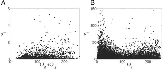
Empirical distributions of even-skipped estimates plotted against observed intensity for each nucleus-pair (A, binomial estimator) or each nucleus (B, Poisson estimator). None of the standard noise models are supported by the empirical distributions.

Open in new tabDownload slide

The main challenge with the binomial estimator is the identification of nuclei pairs. Although the discriminations are reasonably clear visually, we found it hard to develop an algorithm that pairs nuclei with satisfactory reliability. We experimented with various algorithms based on the distance between nuclei, as well as the intensity of the image between nuclei. The latter makes sense because some nuclei pairs that have recently divided remain connected by visible filaments. However, the distances between a correct nucleus pair and an incorrect nucleus pair can be as little as a pixel or two. Given uncertainties in the segmentation of nuclei from the image and determination of the centroids or boundaries, this margin is too thin to be reliable. Further, in some cases, the correct partner for a nucleus is not the nearest one, but the second or third nearest. However, this only becomes clear in the context of the other nuclei in the area. Perhaps further effort could yield a satisfactory algorithm, but we leave this as a topic for future research.

A caveat to both techniques is that they attempt to estimate only the number of fluorescing molecules. If labeling succeeds for only a fraction of proteins, or in the case of more complicated processes such as the formation of inclusion bodies (Iafolla et al., 2008), the number of fluorescing proteins can be significantly less than the total number of proteins present, and either method will underestimate the true amount of protein present.

6 CONCLUSIONS

We have introduced two estimators of protein copy number that apply to still fluorescence expression images with clearly identifiable nuclei or cells. Using these approaches, we estimated copy numbers for 14 genes in the segmentation network of Drosophila. Estimates ranged from several hundreds of proteins per nucleus up to thousands. We consider that these estimates lower bounds, as they assume all variability in expression is due to fundamental stochastic chemical processes. Other sources of noise in the data, which we believe to be present but which did not follow any clear patterns, are expected to drive these estimates lower than true copy numbers. Calibration experiments could resolve how great this bias is, and possibly provide a correction that could allow unbiased estimation of protein copy number in the future.

ACKNOWLEDGEMENTS

L.Z. would like to thank Gregory Butler for encouragement and advice. T.P. thanks Johannes Jaeger, David McMillen and Peter Swain for discussions and feedback that improved this work.

Funding: Department of Computer Science at Concordia University (to L.Z.); Ottawa Hospital Research Institute (to T.P.), McGill University (to T.P.); Natural Sciences and Engineering Research Council of Canada (to T.P.).

Conflict of Interest: none declared.

REFERENCES

Author notes