Large-scale computation of elementary flux modes with bit pattern trees Free

Abstract

1 INTRODUCTION

Systems biology investigates a biological system as a whole because characterizing and understanding single parts or subcomponents often is not sufficient to explain the system behavior. Developing mathematical models for such large-scale systems, however, is a major challenge. Various modeling approaches have been used for studying biological networks to understand interactions at different levels. However, simple approaches like graph analytical methods may lack behavioral predictability and significance (Arita, 2004). Detailed (e.g. deterministic or stochastic dynamic) modeling is mainly limited by insufficient knowledge on mechanisms and parameters (Klamt and Stelling, 2006). At an intermediary level, constraint-based approaches exploit that reaction stoichiometries are often well known even for genome-scale metabolic networks. They gain popularity, for instance, because they allow to predict fluxes for various organisms using linear or quadratic programming (Price et al., 2004).

Constraint-based modeling starts with the m × q stoichiometric matrix ⁠, with q reactions as columns of ⁠, each converting some of the m metabolites (negative entries) into others (positive entries). Thermodynamic conditions constrain the flux rates of irreversible reactions to non-negative values. Since every reversible reaction can be decomposed into two irreversible reactions, we get

(1)

where represents a flux distribution or flux mode. A common assumption is furthermore that the system is in steady state because metabolism usually operates on much faster time scales than the corresponding regulatory events. At steady state, production and consumption of metabolites are balanced and concentrations of (internal) metabolites remain constant:

(2)

Equations (1) and (2) constrain the solution space for possible flux modes to a polyhedral cone called flux cone (see Section 2.2 for formal definitions). Optimization techniques such as flux balance analysis (FBA) define objectives, for instance maximizing for growth or energy production, to predict a single flux distribution (Schuetz et al., 2007). Related methods such as minimization of metabolic adjustment include (experimentally derived) reference flux values to predict the adjustment under different conditions or of knockout mutants (Segrè et al., 2002).

For comprehensive analysis of metabolic network behavior, however, the entire flux cone has to be considered. Minimal functional pathways—elementary flux modes (EFMs)—are desired, into which all operational modes of the network can be decomposed. Moreover, EFMs constitute a unique set of generators for the flux cone (Gagneur and Klamt, 2004). They correspond to extreme rays of the polyhedral cone. Computing EFMs is equivalent to the extreme ray enumeration problem from computational geometry. Most algorithms are variants of the double description method (Motzkin et al., 1953) and for EFMs, two versions are most relevant: the canonical basis approach by Schuster and Hilgetag (1994) and the nullspace approach by Wagner (2004). However, little is known about the complexity of the algorithm, and it is not known whether an algorithm exists with running time polynomial in the input and output size. According to empirical observations, the running time is approximately quadratic in the output size. Unfortunately, the number of EFMs grows exponentially with network size, which currently restricts the application to small- and medium-scale networks of limited connectivity.

Many aspects have to be considered for any successful implementation of an EFM algorithm. After summarizing the most recent and in our opinion the most relevant achievements in Section 2.1, we provide terminology and fundamentals in Section 2.2. The standard implementation of the EFM algorithm with important crunch points is discussed in Section 2.2. In Section 3.1, new methods are introduced, starting with bit pattern trees (Terzer and Stelling, 2006) and its advancement, recursive enumeration of adjacent rays. A new rank updating method using residue arithmetic is developed, and we show how to exploit multi-core architectures of modern CPUs with bit pattern trees. Finally, we demonstrate the power of the new concepts for comprehensive network analysis of Escherichia coli and Helicobacter pylori metabolism (Sections 3.2 and 3.3).

2 METHODS

2.1 Overview

The concept of EFMs for biochemical reaction networks was introduced by Schuster and Hilgetag (1994). The solution space for feasible flux modes shapes a polyhedral cone, thus, extreme ray enumeration algorithms from computational geometry can be used to compute a minimal generating set for the solution space. For EFM computation, variants of the double description method (Motzkin et al., 1953) are most often used. The complexity of the algorithm is poorly understood, but it performs quite well especially for degenerate cases (Fukuda and Prodon, 1995). Performance and memory requirements are both critical for difficult problems. Apart from constraint ordering (see Section 2.3.3), initial matrix and number of iterations have most influence on performance. Mainly geared for EFM computation, Wagner (2004) proposed to use a nullspace initial matrix, leading to algorithm simplifications and improved performance. Subsequently, Gagneur and Klamt (2004) proposed to use binary vectors to store flux values of processed reactions (see Section 2.3.2). This binary approach not only reduces memory demands, but also facilitates set operations during elementarity testing (see Section 2.3.1), another performance-critical aspect of the algorithm. Klamt et al. (2005) use rank computations to test elementarity, and they outline a divide and conquer strategy for parallel computation. In Terzer and Stelling (2006), we introduced bit pattern trees as indexing technique for optimized searching of subsets during elementarity testing. Furthermore, we introduced the concept of candidate narrowing, which is extended here by a new recursive enumeration approach (see Section 3.1.2).

2.2 Definitions

Definition 1.

A set C of points in  R  ^d  is convex if the line segment between any two points in C lies in C. A set C is called a cone if for every⁠, its non-negative multiple lies in C. Combined, we have a convex cone iff

Definition 2.

A convex cone P is called polyhedral cone if it is defined as the solution set of finitely many linear equalities and inequalities, that is, as the intersection of a finite number of hyperplanes and halfspaces:

Definition 3.

A vector    of a polyhedral cone P is called ray if  

 Two rays    and    are equivalent, i.e.  ⁠, if for some α>0.

Theorem 1

(Minkowski's Theorem for Polyhedral Cones). For every polyhedral cone

there exists somesuch that it generates P:

Every ray of the cone is a non-negative combination of columns in ⁠. If we require to be minimal, the columns in are called extreme rays. Minimality or elementarity of rays is essential for the algorithm. Hence we need a formal definition for extreme rays, which is derived in the remainder of this section. We exploit the special structure of the flux cone, leading to simpler definitions and with it often to simpler algorithms.

Definition 4.

Given the stoichiometric matrix  ⁠, the flux cone is a polyhedral cone defined as

A rayof the flux cone is called flux distribution or flux mode, extreme rays are called elementary flux modes or extreme pathways.

The flux cone coincides with the solution space for the constraints given by Equations (1) and (2). Distinctions between EFMs and extreme rays arise from slightly different treatments of reversible reactions [see Wagner and Urbanczik (2005) for exact definitions]. Here, we use the general term extreme rays, assuming that all reactions are irreversible (reversible reactions are already decomposed). The inequality matrix (⁠ in definition 2) is an identity matrix for the flux cone, leading to the subsequent specialized definitions. General definitions for arbitrary polyhedral cones are given in Fukuda and Prodon (1995).

Definition 5.

For any ray  ⁠, the set with indices i corresponding to zero fluxes inis called the zero set of⁠:

Definition 6.

Let    and    be rays of F. If one of the following holds, both hold and    is called an extreme ray:  

• a)

• b) there is nowithother than

 where q is the number of reactions and are the columns of corresponding to non-zero fluxes, represented by ⁠.

2.3 Double description method

Most algorithms for EFM computation are variants of the double description method invented by Motzkin et al. (1953). Starting with an initial cone that contains the final cone, some constraints are already considered and the remaining constraints are iteratively added. Each constraint is represented by a halfspace, which is intersected with the intermediary cone (Fig. 1). The intersection removes some of the extreme rays. New extreme rays are created from adjacent kept/removed extreme ray pairs using Gaussian elimination. The newly created extreme rays lie in the hyperplane separating kept from removed rays. Wagner (2004) proposed a special form of the kernel (or nullspace) matrix of as an initial cone, namely ⁠, where is the identity matrix. If has full rank m, the kernel matrix has dimensions q × (q−m) and consequently m × (q−m). All steady-state constraints (Equation 2) are satisfied by the nature of the kernel matrix. Furthermore, q−m irreversibility constraints (Equation 1) are fulfilled due to the identity matrix in K, leaving m inequalities to be solved in the iteration phase. Inequality constraints of the flux cone involve only one variable, the reaction for which only positive flux values are desired. Let us assume that we are in the iteration phase and have already considered j irreversibility constraints. To add constraint j+1, extreme rays of the flux cone F_j are partitioned into three groups, ⁠, and ⁠, which correspond to rays with positive, zero and negative flux value at reaction j+1, respectively. Extreme rays of the cone F_j+1 are those in and plus new extreme rays generated from ray pairs ⁠. New rays are created by canceling out the flux value at position j+1 using Gaussian elimination, i.e.

(3)

Note that the new ray is a non-negative combination of old rays, and thus by definition 1 surely a ray of the cone. Combining all elements of would generate a quadratic number of new rays measured in terms of intermediary extreme rays. However, only pairs of adjacent rays generate extreme rays (a and g in Fig. 1), thus adjacency testing or better directly enumerating adjacent rays is essential for any feasible implementation.

Fig. 1.

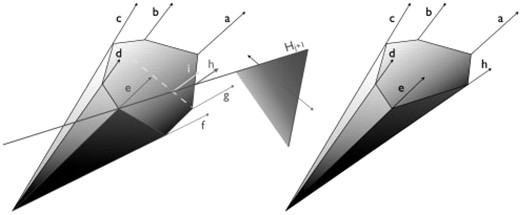
Iteration step of the double description algorithm. A new extreme ray h is created from adjacent rays a and g. Descendants of non-adjacent rays, such as i from c and g, are not extreme rays.

Open in new tabDownload slide

2.3.1 Elementarity testing

Principally, one could use the definition of extreme rays to test elementarity of newly generated rays. Hence, either the rank of a submatrix of is computed according to definition 6a, or the new ray is tested against all other extreme rays as imposed by 6b. Instead of constructing new rays first to discard most of them via the elementary test, it is advantageous to know about elementarity of the new ray beforehand. Only adjacent extreme rays generate new extreme rays, and the definition of adjacency descends from definition 6.

Definition 7.

Both (a) and (b) can be used to test adjacency of two extreme rays. Test (a) does not depend on the number of intermediary extreme rays and thus is not decelerating during computation, which is advantageous. Furthermore, it can be easily applied for distributed computing since it only depends on the rays to be tested and on the stoichiometric matrix—a system invariant. Klamt et al. (2005) actually suggest using the rank test for that purpose. However, for larger networks, rank computation time is not negligible, especially if exact arithmetic is used. It is a cubic algorithm using Gaussian elimination, i.e. O(mm(q−m)) for a full-rank stoichiometric matrix ⁠. In Section 3.1.3 we suggest a new rank update method that circumvents these problems and makes (a) a competitive strategy especially for large networks. Apart from that, it is worth mentioning that rule (a) constrains the minimum number of elements in to ⁠, and it is always a good idea to check this condition first.

2.3.2 Data structures and compression

Zero sets (definition 5) can be implemented as bit sets using one bit per set element. This requires only little space in memory, and set operations such as intersection and union can be computed with bitwise and/or functions—a single CPU operation for set sizes 32(64). Subset (superset) testing is not as obvious, but can be easily derived from the following basic set property:

(4)

Gagneur and Klamt (2004) showed that storing only binary values for processed reactions is sufficient. Intermediary extreme rays consist of a binary and a numeric part. After enforcing irreversibility constraints, flux values corresponding to the processed reaction are converted from numeric to binary. Consequently, only binary extreme rays are left after the last iteration step, from which numerical flux values can be reconstructed.

Another important technique to reduce the size of data structures is to remove redundancies beforehand. This saves memory, but also affects performance since operations on smaller structures are faster, and compacted stoichiometric matrices typically lead to fewer iteration steps. Good overviews of compression techniques are given in Gagneur and Klamt (2004) and in the Appendix B of Urbanczik and Wagner (2005).

2.3.3 Constraint ordering

The double description algorithm is known to be very sensitive to constraint ordering. In Fukuda and Prodon (1995), different row ordering heuristics are compared, favoring simple lexicographical ordering of matrix rows. Using the nullspace approach, the kernel matrix in row-echelon form serves as initial extreme ray matrix. The identity part of the matrix has to be preserved, but remaining rows can (and have to) be sorted to optimize performance. Unfortunately, no mathematical insight is available so far. In practice, we observed good performance with the following orderings: maximum number of zeros (mostzeros), lexicographical (lexmin), absolute lexicographical (abslexmin), fewest negative/positive pairs (fewestnegpos, reducing the set of adjacent pair candidates) and combinations thereof.

3 RESULTS

3.1 Algorithmic improvements

3.1.1 Bit pattern trees

In the iteration phase of the double description method, new extreme rays are generated from adjacent ray pairs. According to definition 7b, we can enumerate all ray pairs and test adjacency by ensuring that no superset exists. This is guaranteed with an exhaustive search over all ⁠, but an indexed search strategy is preferable. Zero sets are q-dimensional tuples, hence multi-dimensional binary search trees (kd-trees) can be used for optimized searching (Bentley, 1975). Therefore, we adapted kd-trees to binary data and invented the concept of bit pattern trees (Terzer and Stelling, 2006).

Figure 2 illustrates superset search on a bit pattern tree. Pseudo code for tree nodes and search method are given in Supplementary Material. The fundamental idea of bit pattern trees is very simple: a binary search tree is constructed, each node separating zero sets containing a certain bit (right child tree) from those not containing the bit (left). Searching a superset of ⁠, we traverse the tree and test at each node whether Z_∩ contains the bit used for separation of zero sets in the subtrees. If Z_∩ contains the bit, only the right child node can contain supersets, if not, both children are recursed.

Fig. 2.

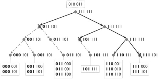
Bit pattern tree with union patterns on the right of every tree node and leaf nodes at the bottom of the tree with zero sets in the boxes. Bold values are common for the whole subtree since they were used to separate left and right tree sets. The set in the dotted box at the top of the tree represents an exemplary intersection set Z_∩. Searching a superset of Z_∩, the tree is traversed along the blue arrows. Dotted arrows are not traversed and truncation of searching is indicated by crosses next to the union pattern causing abortion.

Open in new tabDownload slide

Since the tree will never contain all 2^q possible sets, not all bits will be used for separation in the nodes. We can exploit this to balance the tree by selecting particular bits at tree construction time. Moreover, we store the union pattern Z_U(T)=∪Z_i for every tree node T, unifying all zero sets Z_i∈T. We can abort searching a superset of Z_∩ at node T if Z_∩⊈Z_U(T).

3.1.2 Recursive enumeration of adjacent rays

The simplest approach to use bit pattern trees enumerates all ray pair candidates and tests adjacency as described in the previous section. However, enumerating all pairs is still an elaborate task in O(n²), where n is the number of intermediary modes. To improve this enumeration step, we construct three bit pattern trees, T⁺, T⁻ and T⁰ for rays with positive, negative and zero flux value for the currently processed reaction, respectively. To enumerate all adjacent ray pair candidates (r⁺, r⁻)∈(T+, T⁻), we perform four recursive invocations on the subtrees of the nodes T⁺ and T⁻ [see Step (i) in Fig. 3].

Fig. 3.

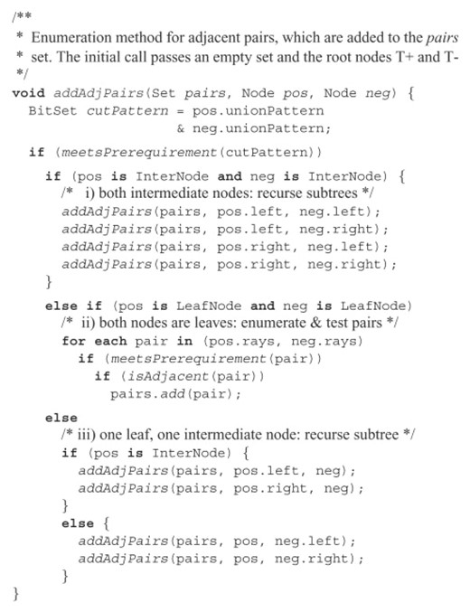
Pseudo code for recursive enumeration of adjacent rays using bit pattern trees. Steps (i) and (iii) contain the recursions, in (ii), adjacent pairs are found and added to the pairs list.

Open in new tabDownload slide

The cut pattern Z_C=Z_U(T⁺)∩Z_U(T⁻) unifies all intersection sets Z_∩=Z(r⁺)∩Z(r⁻), and hence can be used as test set covering all candidates of the subtrees (Terzer and Stelling, 2006). Note that meetsPrerequirement is called on each recursion level, and thus efficient tests are preferable. Any necessary condition for adjacency can be used. Here, we applied minimum set size deduced from adjacency test 7a. A recursion occurs if at least one tree node is an intermediary node. If both nodes are leaves, all pairs are tested, first again using meetsPrerequirement and then by testing for adjacency. If the combinatorial test 7b) is used to implement is Adjacent, we search for supersets in all three trees T⁺, T⁻ and T⁰ (see Supplementary Material for a simple case study).

3.1.3 Lazy rank updating

Instead of the combinatorial adjacency test, as explained in the previous section, we can use the rank test 7a. This has the advantage that testing does not depend on the number of intermediary modes and easily allows for distributed computation. However, for large networks, rank computation is an expensive procedure and some care has to be taken.

Considering that we are recursively traversing two trees with little change between two recursion steps, we can think of an update strategy for the examined matrix. Using Gaussian elimination to compute an upper triangular matrix to derive the rank, we extend the triangular part with every recursion step. Lower recursion levels can then benefit from the precomputed matrix part and only need to perform triangularization of the remaining part.

Let us consider two consecutive recursions of addAdjPairs with parent nodes (P⁺, P⁻) and child nodes (C⁺, C⁻), e.g. assuming the first recursion of Step (i) in Figure 3. Descending the tree, union patterns can only have fewer or equally many elements. Thus, the parent cut pattern is a superset of the child cut pattern, i.e. C_P⊃C_C. Adjacency test 7a consists of two parts: the rank of a column submatrix of ⁠, and the size of the test set ⁠. Here, T coincides with the cut pattern, and since the child set C_C contains at most all elements of C_P, the submatrix contains at least all columns of ⁠. The elements C_C\C_P=C_P\C_C are thus exactly those columns which are added to the triangularized part of the matrix at this recursion step. A single step of the rank update method is illustrated in Figure 4.Note that adjacent enumeration aborts early for many node pairs due to the meetsPrerequirement test. Therefore, we execute triangularization of the matrix lazily, that is, not before a real rank computation is requested.

Fig. 4.

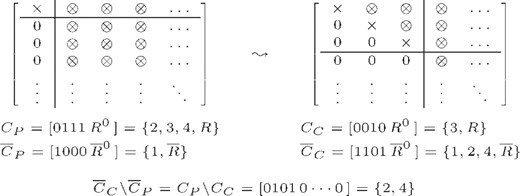
One step of the rank update method: partially triangularized matrix before the current step (left) and continuation after triangularization of columns two and four (right). × stands for non-zero pivot elements, ⊗ for any value. Triangularized columns are reflected by elements in the complementary cut patterns C_P and C_C, respectively. Exemplary patterns are given in binary (square brackets) and standard set notation (curly brackets), R stands for any remainder of the sets, R⁰ for its binary representation. Note that column three and four are swapped during the update step to put the pivots in place, and rows might have been swapped to find non-zero pivot elements. If all remaining elements of an added column are zero, it is put to the end of the matrix and ignored at subsequent steps.

Open in new tabDownload slide

3.1.4 Floating point versus exact arithmetic

Gaussian triangularization with floating point numbers typically uses full pivoting to minimize numeric instability effects. Rank updating uses the same matrix for various rank computations, and instability becomes a serious issue. To circumvent this problem, the non-triangularized matrix part is initially stored at each update level. It is restored before each rank computation and before branching to the next update level. Neglecting that this procedure uses some more memory, it has still two main disadvantages: (i) restoring significantly affects performance, and (ii) instability might still be an issue for large or ill-conditioned matrices.

Rank updating was therefore implemented with exact arithmetic, using rational numbers with large integer numerators and denominators. Opposed to the floating point variant, small pivot elements are chosen to avoid uncontrolled growth of integers. The downside of fraction numbers is 2-fold: arithmetic operations such as addition and multiplication are much more expensive, and integers are possibly still growing, even if fractions are continually reduced. Using store and restore as described for floating point arithmetic improves control of integer growth and leads to better overall performance.

3.1.5 Rank computation using residue arithmetic

A powerful method to implement rank computation is to work with integer residues u modulo a prime m. The residues u are constrained to the interval 0≤u<m using unsigned, and to −m<u<m with signed arithmetic (Knuth, 1997, Section 4.3.2). Assuming that the stoichiometric matrix is rational, we compute the residue matrix by multiplying each numerator n_ij with the multiplicative inverse of the denominator d_ij (modulo m), that is, n′_ij=((n_ij mod m)(d_ij⁻¹ mod m) mod m). Note that multiplicative inverses are defined for numbers being coprime with m. They are computed using the extended Euclidean algorithm. If any of the denominators is not coprime with m, that is, it is a multiple of the prime—which is actually very unlikely for large primes—we multiply the whole column of the matrix with m (or a power of it if necessary) and reduce the fractions.

For the triangularization of the matrix, no inverses are needed. Suppose we have chosen pivot element n′_rc. The new values n″_ij of subsequent rows are then calculated as

resulting in zeros for values n″_ic below the pivot element. If we want to use CPU arithmetic operations, the difference of two products in the above equation has to fit into a register, that is, it has to be below 2^e with e=32(64). We can ensure this by choosing our prime ⁠.

Suppose that we have reached the point where no non-zero values are left when scanning for the next pivot row/column. This is where rank computation normally stops, but in the residue case, one of the zero elements could theoretically be a multiple of our prime, unequal to zero in the non-residue world. That is, the rank computed by residue arithmetic is at most equal to the real rank. The probability of any non-zero value being zero (mod m) is m⁻¹, which could cause a problem if many different rank computations were executed. The probability can be improved to ∏m_i⁻¹ by simultaneously computing the rank for different primes m_i, which can indeed be performed in parallel in modern processors by using SIMD instructions (single instruction multiple data, e.g. SSE instructions of an Intel processor). However, in practice, even a single small prime around 100 did a perfect job.

3.1.6 Exploiting multi-core CPUs

Most current processors have multi-core architectures, allowing multiple threads or processes to run concurrently. We made use of this extra power with the help of semaphores at Step (i) in Figure 3. The semaphore maintains a set of permits, one per CPU core, with efficient, thread safe operations to acquire and release permits. The algorithm tries to acquire a permit to start a new thread. If the permit is received, the four recursive invocations are split into two parts—two invocations for the current, two for the newly created thread. If no permit is acquired, the current thread executes all four recursions. If a thread completes by reaching the leaves of the tree, it releases the permit, triggering a new thread to start soon after. Note that it is important to have very efficient acquire and release operations since they are called very often. The second critical point is the concurrent write access to the pairs set. Either the set itself is made thread safe, or the new thread gets its own set and the parent thread is responsible for merging after completion of the child thread. This dynamic concurrent tree traversal strategy can be improved by primarily collecting recursive invocations to a certain recursion depth if permits are available. A new thread is started for each available permit and all threads concurrently process the collected recursions. Noteworthy, this fine-grained parallelization technique is applicable to both adjacency test variants. It can be applied simultaneously with other parallelization approaches, for instance, the coarse-grained approach given in Klamt et al. (2005) where the computational task is divided into disjunct subtasks that can be run in parallel.

3.2 Benchmarks

For benchmarking, we analyzed an E.coli central metabolism network with 106 reactions and 89 metabolites that was also used in (Klamt et al., 2005). All tests were performed on one or two dual-core AMD Opteron processors of a Linux 2.6.9 machine, using a Java 64-Bit runtime environment (version 1.6.0) with 30 GB maximum heap memory size. For all tests, only the iteration cycle time of the algorithm was taken, excluding preprocessing (compression, etc.) and post-processing (from binary to numeric EFMs). Computation times for the different algorithmic strategies are compared in Figure 5A. Combining recursive enumeration of adjacent rays on bit pattern trees and a combinatorial adjacency test shows best performance for the selected examples. Standard rank computation combined with recursive enumeration of adjacent rays and rank updating with residue arithmetic have similar performance for these examples. The superiority of the rank test in Klamt et al. (2005) may be caused by their unoptimized linear search method for the combinatorial test. Here, we make use of pattern trees for an optimized search (Terzer and Stelling, 2006). However, rank tests might be more efficient for larger networks, since rank testing decelerates probably much slower with increasing stoichiometric matrix size than combinatorial testing, which depends on the exponentially growing number of intermediary modes. For larger networks, we observed better performance for the rank updating method (data not shown). Rank updating is definitely a good choice especially if parallel computation is considered. We recommend residue arithmetic for matrix rank computations in parallelized versions, but rank updating performs remarkably well when exact arithmetic is used instead. Speedup factors for one, two and four threads using two dual core CPUs are shown in Figure 5B. Exploiting multi-core CPUs is particularly effective for large problems, where the speedup factors approach the optimum. For our examples, all methods—even exact arithmetics for the large problems—are faster than CellNetAnalyzer/Metatool (Klamt et al., 2005). For 507 632/2, 450 787 EFMs, we timed 2 min 57 s/92 min 09 s for Metatool (5.0.4) and 1 min 30 s/19 min 39 s for the combinatorial test with one and 40 s/8 min 08 s with four threads, respectively (see Supplementary Material for network configuration details and all computation times).

Fig. 5.

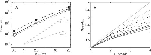
Benchmark results on a system with two dual-core AMD Opteron processors for different configurations for an E.coli central metabolism network. (A) Computation times with four threads for combinatorial test (–·o·–), standard rank test (··×··), rank updating with exact arithmetic (–▪–) and with residue arithmetic (–□–). Dashed gray lines indicate linear and quadratic computation time. (B) Speedup with two and four threads compared to single thread computation. Line colors indicate the problem size: red, blue and black stand for 0.5, 2.45 and 26 Mio EFMs, respectively. Line styles correspond to different computation methods: combinatorial test (—), rank updating with exact arithmetic (…) and with residue arithmetic (– –). The thin gray diagonal represents ideal speedup.

Open in new tabDownload slide

3.3 Large-scale EFM computation

For our first large-scale computational experiment, we used different configurations of the central metabolism network of E.coli (Stelling et al., 2002) with growth on glucose. Besides uptake of glucose, six central amino acids from different biosynthesis families are available, only one at a time in a first experiment. This results in six sets of elementary modes for the amino acids alanine, aspartate, glutamate, histidine, phenylalanine and serine. The sets contain between 321 431 (alanine) and 858 648 (glutamate) EFMs. In a second evaluation, we computed the set of EFMs for combined uptake that consists of 26 381 168 modes.

Figure 6A shows the number of elementary modes per amino acid uptake configuration in terms of the number of simultaneously enabled uptake reactions. The total number of EFMs with at most one amino acid uptake is 1 714 691, only 6.5% of the EFM set enabling simultaneous ingestion of up to six amino acids. Conversely, by computing EFM sets for one amino acid uptake per simulation, and combining the resulting sets afterwards, adding up to 1.7M EFMs, simultaneous uptake cases are missed. These correspond to>90% of the metabolic pathways.

Fig. 6.

(A) Number of EFMs for different amino acid uptake configurations, namely modes without biomass production (nb) and modes with 0–6 concurrently enabled amino acid uptake reactions. Only EFMs on the left of the dashed line can be computed from single amino acid uptake configurations. (B) CV for reaction fluxes of different uptake configurations, considering only top yield EFMs. The configurations are: glucose without amino acid uptake (dashed line), with phenylalanine (dotted), with glutamate (dash-dotted) and with all selected amino acids (solid line).

Open in new tabDownload slide

A major disadvantage of single-objective optimization techniques such as FBA is the restriction to one optimal flux mode. Robustness reflected by a certain degree of flexibility is disregarded. We therefore analyzed flux variability for modes with suboptimal biomass yield (Fig. 6B). We observed no flux variation for zero deviance from the top biomass yield since single EFMs reach optimality. With increasing suboptimality, the number of reactions with coefficient of variation (CV) over 50% grows rapidly. Around 2% below top yield, reaction variation reaches a saturation point. Interestingly, we find a similar saturation point for different CV threshold values (see Supplementary Material for other thresholds). Hence, the cell can achieve high flexibility (robustness) with only little decrease in metabolic efficiency.

Next, we applied our methods to a possibly more realistic, genome-scale metabolic network of H.pylori. In their study, Price et al. (2002) computed the much smaller set of extreme pathways (EPs) for the formation of all non-essential amino acids and ribonucleotides. Here, we focus on the amino acids and compute EFMs for all non-essential amino acids simultaneously. Allowable inputs are d- and l-alanine, arginine, adenine, sulfate, urea and oxygen; outputs are ammonia, carbon dioxide and the carbon sinks succinate, acetate, formate and lactate [in correspondence to case 4 in Price et al. (2002)], together with all non-essential amino acids. Focusing on the production of a specific amino acid, only a small fraction of EFMs is found with typical small-scale simulations, preventing the simultaneous production of other amino acids (between 3% for proline and 16% for asparagine, respectively). Altogether, only 815 576 of 5 785 975 EFMs are found with single amino acid simulations—as for the E.coli case, over 85% of the modes are missed (see Supplementary Material for details). Furthermore, allowing for simultaneous production of all amino acids yields EFMs with larger path lengths as shown in Figure 7 for glycine production. Path length distributions are similar for the other amino acids (see Supplementary Material) and the more complex pathways are not reflected in simplified single amino acid experiments. Hence, our computational methods allow for investigation of combined production of amino acids at a genome-scale level for the first time. Still, applicability to larger networks and more complex environmental conditions has to be shown.

Fig. 7.

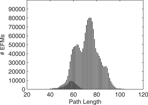
Path length distributions of EFMs for glycine production in H.pylori when glycine is produced alone (dark bars) or possibly jointly with other amino acids (light bars).

Open in new tabDownload slide

4 CONCLUSION

Currently, the computation of EFMs is restricted to metabolic networks of moderate size and connectivity because the number of modes and the computation time raise exponentially with increasing network complexity. Here, we introduced new methods which are several times faster than traditional algorithm variants for medium problem sizes, and even higher speedups are expected for larger problems. We proved the efficiency by successfully competing with alternate implementations, and through large-scale computations for example networks. However, it remains open whether EFMs can be computed for the most recent genome-scale networks. It can possibly be achieved in the near future with intelligent modularization strategies and parallelized algorithms. Memory consumption becomes a major challenge and one might have to consider out-of-core implementations that store intermediary modes on disk. The current in-core implementation requires a lot of memory for large computations. However, our examples with up to 2.5 M EFMs can be run on a normal desktop computer with 1–2 GB memory. We anticipate that porting the code from Java to C will result in rather marginal performance and memory improvements at the cost of reduced interoperability and maintainability. We therefore prioritize out-of-core computation and parallelization. We already applied fine-grained parallelization by exploiting multiple cores of modern CPUs and our rank update method with residue arithmetic is readily applicable to parallel computation. Coarse-grained parallelization complements our multi-core technique and can be applied simultaneously.

To investigate the potential of large-scale EFM computation to yield new biological insight, we first focused on the analysis of E.coli central metabolism. The enhanced computation potential enabled the calculation of over 26 million elementary modes for growth on glucose and simultaneous uptake of selected amino acids. Only a small fraction of these EFMs and none of the maximum yield modes are found with typical small-scale computations. Next, we analyzed the CV for all reactions. Interestingly, flux variation increases rapidly when gradually decreasing optimality of biomass production to 2% below maximum yield. After this saturation point, we observed only little gain of variation. This gives a marginal value where the cell can easily gain robustness at a small price of biomass production. Importantly, such multi-objective flux phenotypes cannot be explained with single objective optimization techniques such as FBA. In a second application, we analyzed the simultaneous production of non-essential amino acids in a genome-scale metabolic network of H.pylori. Most of the more than 5 million EFMs generate multiple amino acids concurrently, and they have significantly larger path lengths than those producing only a single amino acid. These more complex cellular functions are missed with simplified setups considering only one amino acid at a time. Altogether, our study shows both the potential and necessity of large-scale computation of elementary modes, an important step toward universal genome-scale applications.

ACKNOWLEDGEMENTS

We thank G. Gonnet and U. Sauer for pointers to methods and for comments on the article.

Conflict of Interest: none declared.

REFERENCES

Author notes