


Abstract
Motivation: RNA secondary structures with pseudoknots are often predicted by minimizing free energy, which is proved to be NP-hard. Due to kinetic reasons the real RNA secondary structure often has local instead of global minimum free energy. This implies that we may improve the performance of RNA secondary structure prediction by taking kinetics into account and minimize free energy in a local area.
Result: we propose a novel algorithm named FlexStem to predict RNA secondary structures with pseudoknots. Still based on MFE criterion, FlexStem adopts comprehensive energy models that allow complex pseudoknots. Unlike classical thermodynamic methods, our approach aims to simulate the RNA folding process by successive addition of maximal stems, reducing the search space while maintaining or even improving the prediction accuracy. This reduced space is constructed by our maximal stem strategy and stem-adding rule induced from elaborate statistical experiments on real RNA secondary structures. The strategy and the rule also reflect the folding characteristic of RNA from a new angle and help compensate for the deficiency of merely relying on MFE in RNA structure prediction. We validate FlexStem by applying it to tRNAs, 5SrRNAs and a large number of pseudoknotted structures and compare it with the well-known algorithms such as RNAfold, PKNOTS, PknotsRG, HotKnots and ILM according to their overall sensitivities and specificities, as well as positive and negative controls on pseudoknots. The results show that FlexStem significantly increases the prediction accuracy through its local search strategy.
Availability: Software is available at http://pfind.ict.ac.cn/FlexStem/
Contact: [email protected]; [email protected]
Supplementary information: Supplementary data are available at Bioinformatics online.
1 INTRODUCTION
RNA has important functions. Understanding and controlling the functions requires knowledge of RNA structures (Walter et al., 1994). The experimental approach to determining RNA structures is expensive and time consuming. Therefore, computational approaches have been developed to predict RNA structures. However, this problem is challenging due to the incomplete knowledge of RNA folding and the computational complexity.
Currently, there are several computational approaches to predicting RNA secondary structures. Among them, the most accurate ones are comparative methods based on multiple sequence alignment (Eddy and Durbin, 1994; Knudsen and Hein, 1999). However, these methods require a collection of homologous sequences to build their model and hence they are not applicable to the prediction of many novel sequence structures (Huang and Ali, 2007).
Minimal free energy (MFE) is a commonly used ab initio method for predicting RNA structure when only a single sequence is available. Dynamic programming is the most widely used method to compute the optimal (MFE) secondary structure (Hofacker, 2003; Zuker and Stiegler, 1981). However, it is still hard to find the MFE structures of pseudoknotted sequences because pseudoknots violate the recursive definition of the optimal score and bring the MFE problem to an NP-hard problem (Akutsu, 2000; Lyngso and Pedersen, 2000). There are also several dynamic programming algorithms proposed to find the MFE structures of pseudoknotted RNA sequences. They usually use simplistic energy models or restrict the types of pseudoknots. Otherwise they will be too inefficient for most practical uses. Another problem for the MFE method is that current incomplete thermodynamic rules and RNA folding kinetics make the MFE solutions that are often not the true ones in reality.
Heuristic methods have also been explored to predicting RNA secondary structures, especially structures with pseudoknots. Those methods are usually based on the local search technique that ‘explores’ the space of feasible solutions in a sequential fashion, moving in one step from the current solution to a ‘nearby’ one (Kleinberg and Tardos, 2005). Although such algorithms commonly provide no guarantee on optimality of a solution, it is still suitable for predicting RNA secondary structures because current optimal solution (MFE) can also not guarantee ‘true’ solution, and pseudoknots render the MFE problem intractable or NP-hard. In addition, local search techniques can use energy models as accurately as possible for they usually have no restrictions on energy models. Furthermore, the local search technique provides a convenient way to model the sequential nature of RNA folding in some way which may compensate for the deficiency of merely relying on MFE to a certain extent.
There are several types of local search or heuristic approaches to predict RNA secondary structures with pseudoknots (Abrahams et al., 1990; Gultyaev et al., 1995; Ren et al., 2005; Ruan et al., 2004). Many of them take stems (not base pairs) as the elements of RNA secondary structures and regard the secondary structures as the combination of stems. In addition, the formation of the secondary structure can be regarded as a stepwise process, where intermediate structures evolve into the native one by subsequent addition of stems. This is allowed because the initiation is the rate limiting step of stem formation: once a few bases of a stem pair with each other, the rest quickly follows (Abrahams et al., 1990; Saenger, 1984). Therefore, for a RNA sequence, its final secondary structure can be constructed by sequentially adding candidate stems to the potential structure. The criterion to select candidate stems is usually the free energy, since it quantitatively describes the structure's stability gaining from forming a new stem and losing from forming a new loop. However, in the process of adding stems, there are often a large number of candidate stems that can decrease the free energy of the current potential structure at the each step. Choosing candidate stems is a challenging problem for the scarce knowledge about RNA folding kinetics. If we always choose the stem that can mostly decrease the energy of current potential structure, it becomes a greedy process (Abrahams et al., 1990). Such method does not always seem to be feasible because it is entrapped in local minima very easily. If we consider all the suboptimal candidate stems in each step, the combinations of suboptimal candidate stems will be too large to handle. Other heuristic strategies such as genetic algorithm (Gultyaev et al., 1995) may be used to skip the local minima but the designing of the range and style of mutation and crossover is also an intricate problem (Higgs, 2000).
In this article, we observe that in most cases the real structure (maybe not the global MFE structure) of a RNA sequence exists in a local search space, which is constructed using our maximal stem strategy and stem-adding rule induced from validation experiments on some reference RNA structures obtained by experimental or comparative methods. Such strategy and rule reflect the property of RNA folding to some extent. In practice, they can be easily utilized for predicting RNA secondary structure and can greatly reduce the stem's searching space. Consequently, we develop a local search algorithm named FlexStem to predict RNA secondary structures with pseudoknots by searching the local MFE structure. Although the local MFE structures are not always the correct ones, experiments show that they are very close to them.
Moreover, to describe the free energy exactly, FlexStem uses an energy model that combines standard pseudoknot-free energy model including full coaxial stacking energy and the pseudoknot energy model which is also used by other well-known algorithms (Dirks and Pierce, 2003; Ren et al., 2005). This model is quite general in describing pseudoknots (Condon et al., 2004).
FlexStem is tested on a large number of sequences taken from Sprinzl, 5SrRNAs, Pseudobase and other reliable resources. Compared with other well-known algorithms, it has good running efficiency and shows better performance in terms of prediction sensitivity, specificity and positive control on pseudoknotted sequences. Moreover, it also offers biological insight into the characteristic of RNA folding to some extent.
2 METHODS
For a given RNA secondary structure, a helical region or stem can be defined as an anti-parallel complementary strand whose length must be ≥2 bp.
Since RNA secondary structure can be regarded as the combination of stems, predicting RNA secondary structure can be considered by the process of selecting appropriate stems from candidate stem pool. Therefore FlexStem can be divided into three elements, (1) the way to construct candidate stems pool (find candidate stems), (2) the rule and algorithm (stem-adding rule and local search algorithm) to search the appropriate candidate stems and (3) the criteria (free energy model) to evaluate candidate stems during the process of local search.
2.1 Finding candidate stems
The common method to find candidate stems is finding all possible stems (Abrahams et al., 1990; Ren et al., 2005). One of the weaknesses of such method is the large number of all possible stems and their combinations (e.g. TMV, a 189 bases sequence, has 4241 possible stems. Therefore the total number of stem combinations will be very large). Furthermore, some small stems in fact cannot appear in the real structures. In this article, we propose a maximal stem strategy to handle this problem.
First, we take all the maximal stems as candidate stems. A maximal stem is defined as the stem with a maximal length (Fig. 1). We can easily find that a maximal stem with N (N >1) bp contains N×(N − 1)/2 possible stems (Fig. 1). In our statistic, the number of maximal stems is almost 1/3 that of all possible stems. Therefore, adopting maximal stems can significantly reduce the amount of stem combination.

Illustration of maximal stem. The left maximal stem (M1) includes 10 possible stems (four 2-bp stems, three 3-bp stems, two 4-bp stems and one 5-bp stem) and the right maximal stem (M2) includes three possible stems.
Second, we use a flexible merging method similar to the previous work (Isambert and Siggia, 2000) to handle the overlapping (i.e. share bases) candidate maximal stems in the process of building potential RNA secondary structures (Fig. 2).

Illustration of merging strategy. Continuous line denotes the candidate stems in the potential structure and dashed line denotes the candidate stem in the candidate pool that will be added to the potential structure. (a) Indicates the situation before adding a new candidate stem to the potential structure. (b–d) indicate the three possible situations after merging.
The flexible merging method finds the proper (minimal or subminimal free energy) merging points in several possible situations when a new maximal candidate stem overlaps with those stems in the potential structure (c.f. Fig. 2). In this way, our flexible merging method can dynamically produce new stems in the process of building the potential structure if required. Therefore, the finally predicted structure is not restricted to the maximal candidate stems. At the same time, noise structures caused by small stems can be significantly filtered out, thus greatly reducing the search space.
More importantly, based on maximal stem strategy, we deduce the rule of stem adding from the reference secondary structures that can further reduce the search space and therefore design our local search method.
2.2 The rule of adding stem
In the stepwise process of adding stems to the potential RNA secondary structure, there are a large number of candidate stems that can decrease the free energy of the current structure at each step. Therefore, choosing candidate stems is a challenging problem.
We may think that at each step we can rank the candidate stems in descending order according to their abilities to reduce the energy of current structure and only consider top-ranking candidate stems. Deciding the number (or range) of candidate stems at each step is the key to this problem: If it is too small, the search space may miss the true structure. If it is too large, the search space will become too large to handle in a reasonable time.
We find a new clue (stem-adding rule) from the reference RNA secondary structures to overcome this problem. To illustrate this clearly we first define four terms to be used in the rest of the article.
Order: The order of a candidate stem is defined as the rank of the ability of this candidate stem in all the candidate stems capable of decreasing the free energy of the current structure. For example, if the order of a candidate stem is 0, this means that this candidate stem is the optimal candidate stem to the current structure, i.e. this stem can decrease the free energy of the current structure the most. If the order is 1, this means this candidate stem is the first-suboptimal candidate stem to the current structure. Therefore we can see that at each step, every candidate stem in the candidate stems pool one-to-one maps to an order. However, the order of the same candidate stem may be different in different steps because the current structure is changing step by step.
Order Set: A given structure can be considered to be predicted if all the stems of the structure were predicted and a stem in the structure was considered to be predicted if the computed folding contained all base pairs of the stem with the exception of at most 2 bp. This definition can help us to understand the following term: order set.
The order set of a structure is an ordered integer set, consisting of all the orders of the candidate stems stepwise, added to the potential structure in the process of constructing the final structure. For example, if a RNA secondary structure has the order set = {1, 0, 6}, it denotes that this structure is constructed by three stems that are sequentially selected and added to the structure through three steps: first we choose the first-suboptimal candidate stem, second we choose the optimal candidate stem and in the last step we choose the sixth-suboptimal candidate stem. It should also be noted that the same structure may have several different order sets.
Perturbation range: The perturbation range (PR) of an order set is defined as the maximal element (order) in this order set. For example, the PR of the order set {1, 0, 6} will be 6.
Minimal perturbation range: Minimal perturbation range (MPR) is defined as the minimal PR in all possible order sets of a structure. For example, if a structure has a total of three possible order sets: {1,0,6}, {2,4,3}, {1,8,2}, the MPR of this structure is 4.
If the MPR of a structure is m (m≥0), it means that to search such structure we need only to consider at most top m+1 candidate stems at each step (including one optimal candidate stem and m suboptimal candidate stems). It is easy to understand if the MPR of a structure, which has four stems, is 0; the order set must be {0, 0, 0, 0}. This means that to search for this structure we need only select the optimal candidate stem at each step. MPR will help us decide the number of candidate stems that should be considered at each step. If we can get the MPR of sequences with known structures, we suppose that those MPRs can be also used to decide the number of candidate stems that should be considered at each step in the process of searching the possible structure of the sequence with unknown structure.
The algorithm to find the MPR of a reference RNA structure and the experimental results using this algorithm are briefly introduced below.
To find the MPR of a sequence with known structure, we begin with a small integer m (e.g. zero) as an initial guess at the MPR. If we can find an order set of PR m for this structure, then it can be determined that the MPR of this structure is m. Otherwise we literately increase m by one each time and search the order set of this structure within the PR (PR=m) until we find an order set for the structure. In this way, we will obtain the MPR and the order set of this structure. The formal description about this algorithm is not described here due to the limitation of the article size.
We used the complete standard free energy model (Mathews et al., 1999; Serra and Turner, 1995) as our criterion to evaluate the candidate stems and randomly selected 10 tRNA sequences and 10 5SrRNA sequences with known secondary structures from tRNA and 5SrRNA database (Sprinzl et al., 1998; Szymanski et al., 2002) as our test set. The MPR and order sets of those sequences are listed in Table 1.
Perturbation ranges and order sets of the test set
| tRNA | Number of stems | MPR | Order set | 5SrRNA | Number of stems | MPR | Order set |
|---|---|---|---|---|---|---|---|
| DA0260 | 4 | 1 | 1, 0, 0, 1 | X12624 | 8 | 4 | 1,4,1,0,0,3,1,4 |
| DL0220 | 5 | 1 | 0, 0, 0, 1, 0 | X00931 | 7 | 1 | 0,0,0,0,1,1,0 |
| DT5090 | 5 | 1 | 1, 0, 0, 0, 0 | U32122 | 8 | 3 | 2,2,0,1,3,0,0,1 |
| DG7740 | 4 | 4 | 4, 3, 4, 1 | NC0065121 | 7 | 0 | 0,0,0,0,0,0,0 |
| DK9350 | 4 | 1 | 0, 1, 0, 0 | M35569 | 7 | 2 | 0,0,2,0,0,1,0 |
| DD8511 | 4 | 1 | 1, 1, 0, 0 | NC0040881 | 7 | 1 | 0,1,1,0,1,1,0 |
| DS3651 | 4 | 2 | 2, 1, 0, 1 | X02242 | 7 | 5 | 0,0,5,0,2,1,1 |
| DX1660 | 4 | 0 | 0, 0, 0, 0 | X02044 | 7 | 1 | 0,1,0,0,0,0,0 |
| DV7521 | 4 | 0 | 0, 0, 0, 0 | M58385 | 8 | 2 | 1,2,2,0,0,2,2,2 |
| DS1141 | 5 | 4 | 0, 0, 0, 0, 4 | U32122 | 8 | 3 | 2,2,0,1,3,0,0,1 |
According to Table 1, MPR of all the test sequences do not exceed five with an average of 1.85. This means that to find the true structure we need only to consider the top six candidate stems at each step, while those structures with MPR above five can be filtered out even though they may have lower free energies (such structures can be regarded as ‘noise’). This indicates the space of searching candidate stems can be greatly reduced. On the other hand, it can also be observed that ‘0’ is in the majority (>55%) in the add orders of those structures. This means that we need only choose optimal candidate stems in most circumstances. We also perform this experiment on a larger test set (including randomly selected 300 reference tRNA structures and 300 reference 5SrRNA structures) and get the similar result (Table 2).
The statistics of MPR on 300 tRNAs and 300 5SrRNAs
| Average length | MPR≤5(%) | MPR≤6(%) | Percentage of ‘0’ in order sets | |
|---|---|---|---|---|
| tRNAs | 70 | 94 | 95 | 65 |
| 5SrRNAs | 120 | 90 | 94 | 61 |
| Average length | MPR≤5(%) | MPR≤6(%) | Percentage of ‘0’ in order sets | |
|---|---|---|---|---|
| tRNAs | 70 | 94 | 95 | 65 |
| 5SrRNAs | 120 | 90 | 94 | 61 |
In addition, though the current standard free energy model we used is more applicable to relatively short sequences (eg. sequences <130 nt), we investigate the MPR on longer sequences. Using standard free energy model, we randomly selected 10 pseudoknot-free sequences with known secondary structures from RNase database (Brown, 1999) as our test set. The MPR and order sets of those sequences are listed in Table 3.
Perturbation ranges and order sets of the longer sequences
| RNase | length | Number of possible maximal stems | Number of stems | MPR | Order set |
|---|---|---|---|---|---|
| Pichia guilliermondii | 189 | 1635 | 7 | 2 | 2,0,1,0,2,2,0 |
| Crematogaster opuntiae | 196 | 1813 | 8 | 7 | 7,5,0,2,0,0,2 |
| Pichia mississippiensis | 232 | 2390 | 9 | 7 | 1,0,0,2,3,0,0,7,7,0 |
| Wickerhamia fluorescens | 232 | 2601 | 8 | 7 | 1,2,7,0,4,0,4,0 |
| Saccharomyces servazzii | 234 | 2538 | 9 | 8 | 0,2,0,0,8,6,8,0,5 |
| Bordetella bronchiseptica a | 243 | 2359 | 10 | 8 | 7,8,8,4,0,0,7,0,0,1 |
| Saccharomycopsis fibuligera | 243 | 2712 | 7 | 8 | 8,7,5,3,0,0,0 |
| Saccharomyces unisporus | 244 | 2797 | 8 | 3 | 0,0,0,0,1,3,3,0 |
| Kluyveromyces polysporus | 256 | 3278 | 9 | 8 | 0,3,2,8,6,7,5,0,8,0 |
| Pichia canadensis | 333 | 5014 | 12 | 9 | 3,3,0,3,6,7,0,0,6,7,8,9 |
aDenotes that we cannot find the MPR of this structure. But we find the relaxed MPR.
As shown in Table 3, the MPR of the longer sequences has a trend of increasing with the length of sequences. There exists an exceptional structure (denoted by ‘a’ in Table 3) whose MPR cannot be found in limited time. The reason, we think, lies in two aspects: first, the number of candidate stems will dramatically increase with the length of sequences; second, current energy models are in fact not very accurate on long sequences.
However, according to Table 3, we find that MPR is still very small compared to the rapidly increased number of possible candidate stems. In addition, a relaxed MPR for this exceptional structure can be used by requiring that a structure that matches at least 90% of the real structure is found. Considering the relatively low prediction accuracy on long sequences of current algorithms, this relaxation should make sense. Moreover, the MPR will be expected to be further decreased with the more accurate energy model and parameters to be used in the future. Taking into account all these reasons it can be expected that the MPR strategy can also help greatly reduce the search space on larger sequences.

Those observations form the stem-adding rule.
Based on this stem-adding rule, the procedure of adding stems can be regarded as a greedy process with limited perturbations at several steps. This rule can be properly utilized to predict RNA secondary structure and can greatly reduce the solution space of the candidate stems. Consequently we design our local search algorithm (FlexStem) based on this heuristic rule.
2.3 Local search algorithm
To some extent, our local search algorithm is similar to the kinetic pathway of RNA folding. It progressively builds the RNA secondary structure by successive addition of maximal stems.
The basic operation of FlexStem is selecting maximal stems from candidate stem pool and adding them to the potential structure step by step until no maximal stem can be added to the potential structure to decrease its free energy. Therefore, we first define a procedure—AddStem(S, T, m, find) to depict such operation.
AddStem has four parameters: S, T, m and find. Let S be the candidate stem pool, T be the potential structure and m be the order of the candidate stem in S that is considered being added to T. If candidate stem with order m can decrease the free energy of T, then we move it from S to T and let find be 1. Else we keep S and T unchanged and let find be 0.
Specifically, FlexStem includes two phases:
The first phase produces the greedy solution. In each step of this phase, we always select the optimal candidate stem until no next stem can be found that can decrease the free energy of the current structure.
| AddStem (S, T, m, find) |
|---|
| 1: for each stem si in Sdo |
| 2: merge si to T : Ti ← T∪{si} |
| 3: compute the free energy Ei ← E (Ti) |
| 4: end for |
| 5: get the order of each stem si in S according to the rank of Ei and suppose the stem sk is the stem whose order is m |
| 6: if (Ek<E(T)) then |
| 7: S←S− {sk} |
| 8: T←T∪{sk} |
| 9: find ← 1 |
| 10: elsefind ← 0 |
The second phase is a procedure of iterative local search in the neighbors of each stem in the greedy structure. In this phase, we add some ‘perturbation’ to each stem in the greedy structure in order to find more stable possible structures. For example, suppose the greedy structure consists of N stems and we want to perturb the n-th (1≤n≤N) stem (the n-th stem that is added to the greedy structure) in the greedy structure. Then in the n-th step of this local search phase we will select the suboptimal candidate stem, while in the other steps we still select the optimal candidate stem. The range of suboptimal candidate stem that we should consider is decided by the MPR, which is defined in Section 2.2. The secondary structure with minimal free energy among all the perturbations is the final predicted RNA secondary structure. The FlexStem algorithm is described subsequently:
| FlexStem Algorithm: |
|---|
| [1] Initialize Step |
| 1: find all maximal stems and put them into the candidate stem pool S0←{s1, s2, …, sn} |
| 2: initialize the structure T0←Φ(there is no stem in I initially) |
| 3: initialize the P ← MPR |
| [2] Greedy Step |
| (Constructing the greedy structure) |
| 1: S←S0, T←T0, find←1 |
| 2: whilefind=1 do |
| 3: AddStem(S,T,0,find); |
| 4: end while |
| 5: Tgreedy←T |
| 6: N ← |Tgreedy|, (|Tgreedy| denotes the number of stems in Tgreedy) |
| [3] LocalSearch Step |
| (Iterative local search) |
| 1: forn from 0 to Ndo(perturbation on each stem in the Tgreedy) |
| 2: form from 1 to P do |
| 3: S←S0, T←T0, find←1 |
| 4: while (find = 1) do |
| 5: if (|T| = n) then |
| 6: AddStem(S,T,m,find) |
| 7: else |
| 8: AddStem(S,T,0,find) |
| 9: end while |
| 10: Tm,n←T |
| 11: end for |
| 12: end for |
| 13: output the structure Tfinal with minimal free energy among all the ultimate structures. (Tfinal ∈ {Tm,n, Tgreedy} and E(Tfinal)=min{E(Tgreedy), E(Tm,n)}, m∈[1, P], n∈[0,N]) |
2.4 Free energy model
In the process of adding stems, FlexStem uses MFE as its criterion to select stems, because it quantitatively describes the structure's stability gaining from forming a new stem and losing from forming a new loop. Therefore, constructing an appropriate energy model is one of the key factors that determine the quality of a prediction.
FlexStem does not depend on a specific free energy model. It supports all types of pseudoknots and may use non-linear free energy functions. Therefore, in order to obtain high quality, we have adopted the following energy models.


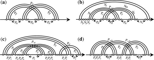
Illustration of the pseudoknots. (a) A Simple pseudoknot. (b) A pseudoknot inside a multiloop. (c) A pseudoknot within a pseudoknot. (d) Overlapping pseudoknots. Nm is the penalty of generating a multiloop, Np is the penalty of the pair in a multiloop and Nn is the penalty of non-paired base in a multiloop. The parameters describing features of these pseudoknots are given in Table 4.
parameters describing features of these pseudoknots
| Symbol | Scoring parameter for | Value(kcal/mol) |
|---|---|---|
| P w | Generating a new external pseudoknot (H-type pseudoknot) | 7.2 |
| P wi | Generating a pseudoknot in a multiloop | 15 |
| P wh | Overlapping pseudoknots | 6 |
| P wp | Pseudoknot in another pseudoknot | 15 |
| P p | Pair in a pseudoknot | 0.1 |
| P n | Non-paired base in a pseudoknot | 0.2 |
3 RESULTS
In this section, we present the prediction results of our algorithm in comparison with the RNAfold (Hofacker, 2003), PKNOTS (Rivas and Eddy, 1999), PknotsRG (Reeder and Giegerich, 2004), ILM (Ruan et al., 2004) and HotKnots (Ren et al., 2005) algorithms. For RNAfold, PknotsRG and HotKnots, the first folding scenario per sequence of the lowest overall energy is selected.
The accuracy of an algorithm is measured by both sensitivity and specificity. Let real pair (RP) be the number of base pairs in the real RNA structure, true positive (TP) the number of correctly predicted base pairs and false positive (FP) the number of wrongly predicted base pairs, we define SE (sensitivity) as TP/RP, and SP(specificity) as TP/(TP+FP). In addition, another two competing criteria (positive control and negative control) are used to quantitatively measure the algorithm's ability to find corrected pseudoknots in pseudoknotted sequences and to avoid finding spurious pseudoknots in unpseudoknotted sequences separately (Dirks and Pierce, 2003).
To illustrate the effect of our local search algorithm in different energy models, tests are divided into two parts. First, we compare the results of FlexStem with exact algorithms under the same or similar pseudoknot-free energy models. Second, using more sophisticated energy model (integrating unpseudoknotted and pseudoknotted models), we compare the results of FlexStem with other algorithms, including exact algorithms and heuristic algorithms.
Finally the efficiency of FlexStem is measured experimentally.
3.1 Prediction results using the same or similar pseudoknot-free energy model as optimal algorithms
To evaluate the effect of our heuristic local search strategy, we first compare the FlexStem (FlexStem 1) with RNAfold (RNAfold1) under the same energy model and parameters [see Equation (1)]. Then we compare the FlexStem (FlexStem2) with RNAfold (RNAfold2) and PKNOTS-1.05 under the similar energy model and parameters [see Equation (2)].
It should be noted that the main difference between the Equation (1) and (2) is that the latter allows coaxial stacking energy. PKNOTS also introduces simplified coaxial energies [similar to Equation (2)] in its dynamic programming program. And for a fair comparison, the PKNOTS is run with pseudoknots prediction turned off.
The test set includes 500 tRNA sequences and 500 5SrRNA sequences randomly selected from Sprinzl tRNA database and 5SrRNA database, separately, which are often used as standard benchmark databases.
As shown in Table 5, FlexStem1 is comparable to RNAfold1 in both sensitivity and specificity with the same energy model (FlexStem even performs better on tRNAs) and FlexStem2 outperforms PKNOTS and RNAfold2 in both sensitivity and specificity on tRNAs and 5SrRNAs. It can also be observed that the coaxial energy seems to be more essential for tRNAs than for 5SrRNAs.
Summary of the testing result on tRNAs and 5SrRNAs
| tRNAs | 5SrRNAs | |||
|---|---|---|---|---|
| SE | SP | SE | SP | |
| RNAfold1 | 63 | 59 | 62 | 61 |
| FlexStem1 | 68 | 67 | 63 | 60 |
| RNAfold2(a) | 71 | 68 | 58 | 56 |
| FlexStem2 | 77 | 73 | 62 | 58 |
| PKNOTS | 72 | 68 | 42 | 40 |
| tRNAs | 5SrRNAs | |||
|---|---|---|---|---|
| SE | SP | SE | SP | |
| RNAfold1 | 63 | 59 | 62 | 61 |
| FlexStem1 | 68 | 67 | 63 | 60 |
| RNAfold2(a) | 71 | 68 | 58 | 56 |
| FlexStem2 | 77 | 73 | 62 | 58 |
| PKNOTS | 72 | 68 | 42 | 40 |
(a) RNAfold2 can allow coaxial stacking energy using –d3 option.
Considering the coaxial stacking energy and multiloop energy FlexStem adopts [see Equation (2)], which are more accurate than many other algorithms, we in addition test FlexStem on this test set using the same simplified energy functions used by other algorithms. From our tests we find that the prediction results of FlexStem, no matter it adopts the more accurate coaxial stacking energy and multiloop energy or the simplified ones, are almost the same. This implies that the current simplification on those two kinds of energies will not decrease the prediction accuracy in practice.
3.2 Prediction results using more sophisticated model
To evaluate the capability of FlexStem in predicting the pseudoknotted sequences we extend the free energy model in FlexStem to support the pseudoknot energy model [see Equations (3) and (4)] and compare FlexStem with other four algorithms (PKNOTS, PknotsRG, Hotknots and ILM) that can deal with pseudoknots.
Experiments are made on pseudoknot-free sequences and pseudoknotted sequences separately. For a fair comparison, the PKNOTS and FlexStem are run with pseudoknots prediction turned on (denoting by a suffix ‘−k’) and PknotsRG-mfe is used.
3.2.1 Prediction results on pseudoknot-free sequences
According to Table 6, FlexStem still shows the best performance in terms of prediction sensitivity (76%) and specificity (69%) on tRNAs. PKNOTS and PknotsRG perform better on overall negative control.
Summary of the testing result on tRNAs and 5SrRNAs
| tRNAs | 5SrRNAs | |||||
|---|---|---|---|---|---|---|
| SE | SP | NC | SE | SP | NC | |
| PKNOTS-k | 75 | 67 | 95 | 40 | 39 | 93 |
| PknotsRG-mfe | 63 | 61 | 92 | 62 | 61 | 90 |
| ILM | 68 | 61 | 76 | 64 | 64 | 80 |
| Hotknots | 66 | 58 | 65 | 61 | 60 | 95 |
| FlexStem-k | 76 | 69 | 90 | 61 | 58 | 89 |
The tRNA database includes 500 5SrRNA sequences. ‘NC’ denotes negative control.
3.2.2 Prediction results on pseudoknotted sequences
The experiments are performed on three datasets. The first dataset (Table 7) includes 25 pseudoknotted sequences in different types from reliable resources.
Detail results on sequences with pseudoknots
| Name | Lens | Pair | HotKnots | ILM | PknotsRG | PKNOTS-k | FlexStem-k | ||||||||||
|---|---|---|---|---|---|---|---|---|---|---|---|---|---|---|---|---|---|
| SE | SP | K | SE | SP | P | SE | SP | K | SE | SP | K | SE | SP | K | |||
| alphamRNA | 112 | 24 | 46 | 30 | 0/1 | 50 | 33 | 0/1 | 46 | 29 | 0/1 | 46 | 33 | 0/1 | 62 | 43 | 0/1 |
| APLV | 83 | 22 | 68 | 60 | 1/1 | 27 | 26 | 1/1 | 86 | 79 | 1/1 | 73 | 70 | 1/1 | 73 | 67 | 1/1 |
| BBMV1 | 116 | 38 | 68 | 68 | 0/1 | 79 | 81 | 0/1 | 53 | 57 | 1/1 | 74 | 72 | 0/1 | 100 | 93 | 1/1 |
| BBMV2 | 114 | 39 | 79 | 82 | 0/1 | 82 | 82 | 0/1 | 77 | 83 | 1/1 | 77 | 77 | 0/1 | 97 | 90 | 1/1 |
| BBMV34 | 114 | 39 | 79 | 82 | 0/1 | 82 | 82 | 0/1 | 77 | 83 | 1/1 | 74 | 74 | 0/1 | 97 | 93 | 1/1 |
| Biotin | 61 | 12 | 83 | 50 | 1/1 | 83 | 53 | 1/1 | 92 | 58 | 1/1 | 58 | 33 | 0/1 | 92 | 58 | 1/1 |
| BMV1 | 134 | 44 | 84 | 86 | 0/1 | 86 | 84 | 0/1 | 84 | 86 | 0/1 | 84 | 80 | 0/1 | 86 | 84 | 0/1 |
| BMV2 | 134 | 44 | 80 | 85 | 0/1 | 86 | 84 | 0/1 | 80 | 85 | 0/1 | 84 | 80 | 0/1 | 86 | 84 | 0/1 |
| BMV34 | 134 | 44 | 84 | 86 | 0/1 | 86 | 84 | 0/1 | 84 | 86 | 0/1 | 84 | 80 | 0/1 | 86 | 84 | 0/1 |
| Bt-PrP | 45 | 12 | 42 | 38 | 0/1 | 42 | 33 | 0/1 | 33 | 27 | 0/1 | 50 | 46 | 0/1 | 100 | 80 | 1/1 |
| CCMV1 | 134 | 46 | 80 | 84 | 0/1 | 80 | 84 | 0/1 | 80 | 84 | 0/1 | 80 | 80 | 0/1 | 82 | 79 | 1/1 |
| CCMV2 | 134 | 46 | 80 | 84 | 0/1 | 80 | 84 | 0/1 | 80 | 84 | 0/1 | 80 | 80 | 0/1 | 82 | 86 | 0/1 |
| CCMV34 | 134 | 46 | 82 | 86 | 0/1 | 82 | 86 | 0/1 | 69 | 70 | 0/1 | 67 | 67 | 0/1 | 84 | 85 | 1/1 |
| CYVV | 85 | 24 | 83 | 77 | 1/1 | 62 | 65 | 0/1 | 83 | 80 | 1/1 | 96 | 92 | 1/1 | 83 | 77 | 1/1 |
| EMV | 80 | 22 | 73 | 59 | 0/1 | 50 | 50 | 0/1 | 73 | 67 | 0/1 | 73 | 62 | 0/1 | 73 | 64 | 0/1 |
| Ec_S15 | 67 | 17 | 100 | 74 | 1/1 | 59 | 62 | 0/1 | 76 | 68 | 1/1 | 100 | 74 | 1/1 | 100 | 74 | 1/1 |
| HDV_anti | 91 | 25 | 20 | 18 | 0/1 | 20 | 17 | 0/1 | 20 | 18 | 0/1 | 44 | 34 | 0/1 | 44 | 34 | 0/1 |
| HDV | 87 | 28 | 43 | 44 | 0/1 | 46 | 43 | 0/1 | 96 | 87 | 1/1 | 86 | 75 | 0/1 | 89 | 74 | 0/1 |
| MMTV | 34 | 11 | 100 | 92 | 1/1 | 0 | 0 | 0/1 | 100 | 92 | 1/1 | 100 | 92 | 1/1 | 100 | 92 | 1/1 |
| T2_gene32 | 33 | 12 | 100 | 100 | 1/1 | 58 | 100 | 0/1 | 100 | 100 | 1/1 | 100 | 100 | 1/1 | 100 | 100 | 1/1 |
| TMV | 189 | 59 | 54 | 64 | 0/4 | 53 | 54 | 0/4 | 54 | 62 | 0/4 | 53 | 61 | 0/4 | 46 | 54 | 0/4 |
| TMVup | 84 | 25 | 52 | 62 | 0/3 | 52 | 65 | 0/3 | 80 | 83 | 2/3 | 52 | 68 | 0/3 | 84 | 78 | 2/3 |
| TMVdown | 105 | 34 | 68 | 74 | 0/2 | 65 | 69 | 0/2 | 68 | 74 | 0/2 | 94 | 94 | 2/2 | 74 | 71 | 1/2 |
| TYMV | 86 | 23 | 70 | 70 | 0/1 | 83 | 70 | 1/1 | 78 | 75 | 1/1 | 100 | 92 | 1/1 | 83 | 76 | 1/1 |
| Tt-LSU-P3 | 65 | 20 | 95 | 100 | 1/1 | 80 | 80 | 0/1 | 85 | 100 | 0/1 | 55 | 61 | 0/1 | 95 | 100 | 1/1 |
| Average SE and SP | 72 | 70 | 7/31 | 63 | 63 | 3/31 | 74 | 73 | 13/31 | 75 | 71 | 8/31 | 84 | 77 | 17/31 | ||
| Positive Control | 23 | 10 | 42 | 26 | 55 | ||||||||||||
‘K’ = (number of correctly predicted pseudoknots). (Ruan et al., 2004)
According to Table 7, FlexStem shows the highest average sensitivity (84%), specificity (77%), as well as the best positive control ability (55%), outperforming the other competitive algorithms.
The second dataset (Table 8) includes the long pseudoknotted sequences from RNases, tmRNAs and 16SrRNAs. According to Table 8, the performances of all the tested algorithms are not so good and are descended with the increase of sequence's length (however, FlexStem still performs better than other three algorithms on the tested sequences). The main reason, we think, lies in that the current energy model and parameters are mostly based on melting studies on short oligonucleotides (Freier et al., 1986).
Detail results on long sequences with pseudoknots
| Name | Lens | Pair | HotKnots | ILM | PknotsRG | PKNOTS-k | FlexStem-k | ||||||||||
|---|---|---|---|---|---|---|---|---|---|---|---|---|---|---|---|---|---|
| SE | SP | K | SE | SP | K | SE | SP | K | SE | SP | K | SE | SP | K | |||
| Methanococcus jannaschii | 252 | 75 | 73 | 72 | 0/1 | 71 | 68 | 0/1 | 69 | 68 | 0/1 | * | * | * | 75 | 71 | 0/1 |
| Acidianus ambivalens | 262 | 75 | 61 | 58 | 0/1 | 73 | 69 | 0/1 | 61 | 58 | 0/1 | * | * | * | 80 | 73 | 0/1 |
| Acidianus brierleyi | 267 | 73 | 62 | 62 | 0/1 | 64 | 63 | 0/1 | 49 | 47 | 0/1 | * | * | * | 67 | 67 | 0/1 |
| Metallosphaera sedula | 304 | 90 | 43 | 41 | 0/2 | 49 | 46 | 0/2 | 56 | 53 | 0/2 | * | * | * | 62 | 62 | 0/2 |
| Aeropyrum pernix | 330 | 106 | 25 | 24 | 0/1 | 45 | 49 | 0/1 | 25 | 24 | 0/1 | * | * | * | 57 | 54 | 0/1 |
| tmRNA.E.coli | 362 | 106 | 49 | 48 | 0/4 | 49 | 48 | 0/4 | 49 | 48 | 0/4 | * | * | * | 41 | 41 | 1/4 |
| 16S.E.coli | 1542 | 478 | 37 | 36 | 0/4 | 37 | 36 | 0/4 | 48 | 48 | 0/4 | * | * | * | 42 | 46 | 0/4 |
| Average SE and SP | 50 | 49 | 0/14 | 55 | 54 | 0/14 | 51 | 50 | 0/14 | * | * | * | 61 | 60 | 1/14 | ||
‘*’ indicates we were unable to run the algorithm to completion.
For a more fair and general comparison, we additionally test five algorithms on third dataset (Table 9). This dataset comes from the PseudoBase, a widely used reliable pseudoknot database (van Batenburg et al., 2000). PseudoBase includes 16 categories of pseudoknots, which include all the pseudoknots used as benchmarks in recent papers (Dirks and Pierce, 2003; Ren et al., 2005; Rivas and Eddy, 1999; Ruan et al., 2004). After excluding the redundant pseudoknots (>85% similarity) and unnatural SELEX pseudoknots the test set includes 168 pseudoknots (denoted by pk168). This dataset was also used by a recent algorithm (Huang and Ali, 2007) as the benchmark dataset.
Summary of testing results on pk168 set (including 168 sequences with pseudoknots)
| SE | SP | Positive control | |
|---|---|---|---|
| PKNOTS-k | 73 | 73 | 48 |
| PknotsRG-mfe | 76 | 71 | 51 |
| ILM | 65 | 60 | 22 |
| Hotknots | 70 | 69 | 33 |
| FlexStem-k | 80 | 72 | 57 |
| SE | SP | Positive control | |
|---|---|---|---|
| PKNOTS-k | 73 | 73 | 48 |
| PknotsRG-mfe | 76 | 71 | 51 |
| ILM | 65 | 60 | 22 |
| Hotknots | 70 | 69 | 33 |
| FlexStem-k | 80 | 72 | 57 |
According to Table 9, FlexStem performs best among the five algorithms in terms of the sensitivity (80%) and positive control (57%). PKNOTS obtains the highest specificity (73%). The experimental results of HotKnots, ILM, PknotsRG and PKNOTS are also consistent with previous results (Huang and Ali, 2007).
3.3 Running efficiency
The FlexStem algorithm is implemented using C++. The experiments are performed on a 2 GHz processor with 2 MB cache size, running Ubuntu Linux. The efficiency of algorithm is evaluated by time and space cost.
According to Table 10, we can see that FlexStem has the minimal memory cost among five algorithms. In terms of the time efficiency FlexStem is comparable to HotKnots and significantly better than PKNOTS. ILM is the fastest one among the five methods.
Performance results for random RNA sequences
| Time (h:m:s) and space (MB) cost | ||||||||||
|---|---|---|---|---|---|---|---|---|---|---|
| Length | ILM | HotKnots | PKNOTS | PknotsRG | FlexStem | |||||
| Time | Mem | Time | Mem | Time | Mem | Time | Mem | Time | Mem | |
| 40 | 0.03 | 0.6 | 0.06 | 1.7 | 14 | 15 | 0.03 | 3.1 | 0.05 | 0.5 |
| 80 | 0.03 | 0.8 | 9.2 | 2.0 | 19:10 | 48 | 0.04 | 6.5 | 3.23 | 0.6 |
| 100 | 0.09 | 0.9 | 12.3 | 2.1 | 1:05:24 | 95 | 0.11 | 7.4 | 6.3 | 0.7 |
| 200 | 0.4 | 1.4 | 55 | 35 | * | * | 1.1 | 9.1 | 41 | 1.1 |
| 400 | 3.1 | 3.4 | 1:45 | 98.4 | * | * | 24 | 14.5 | 1:31 | 1.6 |
| 800 | 16.3 | 12.5 | 24:24 | 112 | * | * | 18:23 | 23.4 | 25:32 | 3.1 |
‘*’ indicates we were unable to run the algorithm to completion for the time or memory limitation on our reference machine.
4 DISCUSSION AND CONCLUSIONS
In this article, we present a heuristic algorithm, called FlexStem, for predicting RNA secondary structures with pseudoknots.
From the algorithmic point of view, FlexStem only searches the local MFE structure in a very limited space. Its improvement on the prediction performance lies in its greatly reduced local space constructed by MPR and this space in most circumstances includes the real structure.
With regard to the pseudoknot model, Hotknots adopts D&P model that is converted from the R&E model used by PKNOTS. PknotsRG uses the csr-PK model which is also simplified from the R&E model, and ILM does not employ any pseudoknot. Based on the previous work (Condon et al., 2004), the classes of the pseudoknot models used by those algorithms can be properly ordered as: PknotsRG⊂HotKnots⊂FlexStem⊂PKNOTS. According to our experiment on pseudoknots, we find that ILM has relatively low prediction accuracy compared to other ones that employ pseudoknot models, which may imply that adopting a general pseudoknot energy model is still important for predicting pseudoknots though thermodynamic information for pseudoknots is scarce at present.
To further probe the effect of perturbation strategies of FlexStem, we also compare the prediction results of FlexStem with greedy structures (structures with no perturbation). We find that though current FlexStem only allows perturbations on one stem, it can significantly increase the prediction accuracy compared to greedy structures (results are described in the Supplementary Material A).
It is obvious that enlarging the range of MPR and the number of perturbation stems in the local search process will help further decrease the free energy of the solution structure. However, it does not mean that the prediction accuracy will simply increase in this way, and what is worse, the prediction accuracy may even decrease on a larger search space. In fact, we have analyzed the prediction results of FlexStem on the pseudoknot-free sets and compared them with the reference structures as well as the optimal (MFE) structures according to their standard free energies. We find that the average free energy of the structures predicted by FlexStem is already smaller than that of the reference structures. The solutions of FlexStem are closer to the reference structures than the optimal solution (MFE) structures from the energy point of view in most of the tests (examples are described in the Supplementary Material B).
The performance of FlexStem may be improved by considering the following factors in the future. The first factor is still the energy models. Second, FlexStem has the potential to further improve the prediction accuracy by allowing simultaneous perturbations on two or more stems in each structure, though designing the efficient search algorithm dealing with such cases is also a challenging problem. In addition, further investigations on current MPR space may help further reduce the local search space, which may not only increase the prediction accuracy but also help provide more insights into the details of RNA folding processes.
ACKNOWLEDGEMENTS
We thank Yan Fu, Haipeng Wang from Chinese Academy of Sciences for their valuable helps and suggestions.
Funding: This work was supported by the National Key Basic R&D Program (973) of China under Grant No. 2002CB713807, Frontier Project of Knowledge Innovation Program of Chinese Academy of Sciences and National Natural Science Foundation of China under Grant No. 90612019 and 60503060.
Conflict of Interest: none declared.
References
Author notes
Associate Editor: Ivo Hofacker

