Mining significant tree patterns in carbohydrate sugar chains Free

Abstract

1 INTRODUCTION

Carbohydrate sugar chains or glycans are the third major class of cellular macromolecules, next to nucleic acids and proteins. Located on the outer surface of a variety of cells, glycans which are usually attached to proteins or lipids play various important roles for interacting with outer molecules and cells, such as molecular recognition in antigen–antibody interactions and signals controlling the fate of cells (Stanley, 2007). However, a lot of biological roles of glycans are still unclear, mainly because glycans hold branch-shaped tree structures or rooted trees (Varki et al., 1999). This unique, complex feature hindered developing useful experimental tools for determining glycan sequences, having resulted in the slow accumulation of glycan sequences. However, due to the recent development of high-throughput experimental techniques such as mass spectrometry (Haslam et al., 2006), databases for sequences of glycans are developing (Hashimoto et al., 2006). Similarly, informatics tools for glycans are also on the way (Raman et al., 2005). For example, a problem of classifying glycans in some class from others attracts machine-learning groups to develop new approaches such as kernel-based methods for this problem (Yamanishi et al., 2007). However, kernel methods such as support vector machines (SVM) have the apparent drawback in incomprehensibility on their results, and it would be more valuable to develop computational methods which can find biologically understandable patterns from the accumulating data.

We address the issue of finding motifs or conserved, significant patterns in glycans which can be visibly understandable and must be helpful for promoting biological findings in glycobiology and related fields. In fact, like sequence motifs in proteins, biologically important, conserved parts in glycans have been already pointed out (Lanctot et al., 2007). As hidden Markov models for protein families and domains, probabilistic models for glycans were already proposed for glycan families and their conserved patterns (Aoki-Kinoshita et al., 2006; Hashimoto et al., 2008). These models work well for aligning multiple glycan trees and find patterns which can be found at almost the same location in different glycans. However, glycan trees are ubiquitous, meaning that conserved patterns can be at different branches or leaves in different trees. In this sense, probabilistic model-based approaches are not necessarily good enough for capturing patterns which appear at totally diverse locations of different glycan trees. Thus, it is urgent to develop a method for capturing conserved, significant patterns which appear in different positions in multiple glycans.

For this issue, we present a well-grounded, efficient method, which has two procedures: mining frequent subtrees from given glycan tree data and checking the significance of frequent subtrees by statistical hypothesis testing.

The first part is based on frequent subtree mining which is an extension of frequent itemset mining, a traditional framework in the field of data mining, to rooted, labeled, ordered trees or simply trees (Zaki, 2002). Frequent subtree mining can be defined as the problem of finding all frequent subtrees from a given large number of trees, where given a set of trees the number of trees containing a subtree T is called the support of T, denoted by support(T), and a frequent subtree is a subtree whose support is larger than or equal to a given cut-off value called minimum support, denoted by minsup. Thus we can expect that a method for mining frequent subtrees is effective for our issue, if we use an appropriate minsup. Practically, however, given glycans, the number of frequent subtrees reaches a very large number, because they are redundant. For this problem, a powerful idea in the literature of data mining is mining closed frequent subtrees and mining maximal frequent subtrees (Chi et al., 2005). A frequent tree T can be defined to be closed unless the support of any supertree of T is equal to that of T, while it can be maximal unless any supertree of T is frequent. More concretely, the idea of closed frequent subtrees allows to remove a redundant subtree if its support is equal to that of any of its supertrees. However, each entry of a glycan database is basically unique, causing a deficient case that the support of a frequent tree is very close to that of its supertree but not equal to. This results in that there still remain a large number of closed frequent subtrees. On the other hand, the idea of maximal frequent subtrees outputs the largest frequent subtrees, resulting in that many frequent subtrees can be summarized into only one maximal frequent subtree. A big problem is that the information on the support of each frequent subtree is lost by this method, meaning that this idea might be too coarse to analyze all frequent subtrees. Thus, to solve these problems, we propose a new idea, α-closed frequent subtrees, where a frequent tree T can be defined to be α-closed unless support(T′)≥max(α × support(T), minsup) for any supertree T′ of T, where α takes a value between zero and one. We further propose a method for enumerating all α-closed frequent subtrees from a given number of trees or glycans, keeping almost the same computational burden of an algorithm for mining closed frequent subtrees. We note that this idea is a natural extension of closed frequent subtrees, relaxing the relatively strong restriction of closed frequent patterns to reduce the redundant patterns more. A further notable, interesting feature is that if α=1, mining α-closed frequent subtrees is mining closed frequent subtrees while it is mining maximal frequent subtrees if α=0. This means that we can adjust α to control the number of frequent subtrees to be generated.

For frequent subtrees which are obtained in the above procedure, the only criterion to rank them is their frequencies, which however might not be good enough, since they are easily biased by the frequencies of monosaccharides. Thus to sift significant patterns from frequent subtrees, we propose to apply statistical hypothesis testing. More concretely, given a glycan dataset, we first generate a control dataset, i.e. trees that are synthetically generated by using the distribution of given glycans, then for each frequent subtree, generate a 2 × 2 contingency matrix representing the number of appearances of this subtree in the given dataset and the generated control dataset and finally perform Fisher's exact test for independence on this table. Fisher's exact test of significance can be applied to any distribution over the table, meaning that it works under the case where an entry of the contingency matrix is zero. With the above procedure, we can rank the frequent subtrees according to P-values of the hypothesis testing and if required, select only the top subtrees.

We further show that the significant subtrees obtained by the above procedure can be applied to classification problems of glycans. For this purpose, we generate a weighted ensemble of classifiers, each of which is a weak learner developed by each significant pattern, and optimize the weight by the maximum margin criterion. An advantage of this method, which is equivalent to ν-SVM with a linear kernel (Schölkopf and Smola, 2002), is that it can clearly show features (significant patterns) that work well for classification.

We empirically examined our proposed method in two different manners: (1) Biological significance of obtained significant α-closed subtrees and (2) comparison of classification performance with other competing methods such as SVM with tree kernels. In the first experiment, we obtained significant subtrees from all entries in the KEGG Glycan database, and examined the top 10 patterns ranked by hypothesis testing from a biological viewpoint. We found that all of them were typical motifs, which could be classified into two types: (1) those which are found at parts relatively close to leaves of glycans and distributed over different glycan classes and (2) so-called ‘cores’ which are subtrees including the root and specific to particular glycan classes. We emphasize that it has been difficult to automatically capture these motifs by computational approaches. In the second experiment, we focused on one class of glycans, O-glycan, and tested the classification performance of our method using 10 × 10-fold cross-validation, comparing with those by SVM with three tree kernels. Experimental results indicate that our method outperformed all three competing methods, being all statistically significant.

2 METHODS

2.1 Preliminaries

A graph has nodes and edges connecting nodes. A tree, which is usually denoted by T, is a graph without any loop. If a tree has a special node called the root, it is a rooted tree. If nodes and edges of a tree are labeled, it is a labeled tree. A leaf or end node is a node which is not the root and has only one edge connecting to this node. Internal nodes are the nodes which are neither leaves nor the root. A node x on a unique path from the root to a node y is an ancestor of node y, where y is a descendant of x. A parent is the closest ancestor, and a child is the closest descendant. If the children of a node is ordered, it is a ordered tree. Children are called siblings, and the first child is called the eldest sibling and the last child is called the youngest sibling. In this article, we regard glycans as rooted, labeled, ordered trees, meaning that all trees in this paper are rooted, labeled, ordered trees, which are hereafter simply called trees. If tree T′ has nodes and edges which form subsets of nodes and edges of tree T, T′ is a subtree of T, and T is a supertree of T′. The subtree of a node is the set of all descendants (with this node) and all edges connecting to these nodes. The size of tree T is the number of edges in T, denoted by |T|. An immediate supertree T′ of T satisfies |T′|=|T|+1.

2.2 Mining α-closed frequent subtrees

2.2.1 Definition

Given a set of trees, the support of a tree T is the number of trees containing T, usually denoted by support(T). A frequent tree is the tree whose support is larger than or equal to a given cut-off value called minimum support, denoted by minsup. A frequent tree is defined to be closed unless the support of its any supertree is equal to the support of this tree. Similarly a frequent tree is defined to be maximal unless any of its supertrees is a frequent tree.

DEFINITION 2.1

PROPERTY 2.1. (Subsets).

PROPERTY 2.2.

PROPERTY2.3.

2.2.2 Enumeration tree

To find all α-closed frequent subtrees, we have to traverse a search space of subtrees, scanning over a given set of trees, and check whether each subtree is α-closed frequent or not. If we check the subtrees randomly, the computational burden is explosively high, and so we need to make this search space efficient enough.

Thus, we use a particular search tree for the search space. We define the rightmost node of a tree as the node which is reached at the end of the depth-first traversal, and the rightmost path of a tree T is defined as the unique path from the rightmost node to the root. Let RMP(T) be the list of nodes on the rightmost path of a tree T from the rightmost node to the root. We can generate a search tree by the following procedures: (1) We start with the root labeled by null, (2) a child of the root is labeled by only one node and (3) for a node labeled by a tree T, its children are labeled by immediate supertrees of T which are generated by extending one edge at all nodes in the rightmost path of T. This search tree, which we hereafter call an enumeration tree, has the following nice property (Asai et al., 2002), and in this article, we use this tree as a search space of subtrees because of its efficiency.

PROPERTY 2.4.

2.2.3 Algorithm

When we traverse the enumeration tree from the root to leaves, if we do no longer have to check the subtree of a node in the enumeration tree, this makes the traverse more efficient. This is called pruning, and the first idea is the downward closure property, which is commonly used in a lot of frequent mining problems:

PROPERTY 2.5 (Downward closure property).

We note that we can apply the downward closure property to each edge of an enumeration tree. That is, we can prune the subtree of a node in an enumeration tree if a tree of this node is not frequent, because of the downward closure property.

We can further prune the enumeration tree by employing an idea usually used in algorithms for mining closed frequent subtrees (Chi et al., 2005) and mining closed frequent subgraphs (Yan and Han, 2003). We define the blanket of a frequent tree T, denoted by B(T), as the set of immediate supertrees of T that are frequent. For T′∈B(T), if w is a node which is in T′ and not in T and v is the parent of w, we write T′← T_v+w and let B(T_v) be the subset of B(T) having immediate supertrees T′ obtained by, fixing v, changing w for all cases. The B(T) can be partitioned into two subsets: the left blanket B_L(T) and the right blanket B_R(T). The B_R(T) can be defined by the set of all T′ (∈B_R(T)) where w, which is in T′ and not in T, is the rightmost node of T′. We note that B_R(T) is the set of children of T in the enumeration tree. The B_L(T) can be defined by that B_L(T)=B(T)−B_R(T).

Two trees T and T′(∈B(T)) are occurrence matched, if at least one T′ appears every time when T appears in a given dataset. For example, given three trees shown in Figure 1, two trees T and T′ corresponding to Figure 2(a) and (b), respectively, are occurrence matched, because T′ appears every time when T appears in the three trees of Fig. 1. Using this concept, we can derive two nice properties, which are important for pruning, as follows:

Fig. 1.

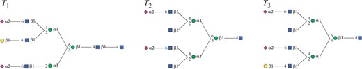
Labeled ordered tree examples.

Open in new tabDownload slide

Fig. 2.

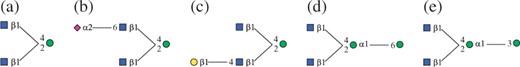
Subtree examples.

Open in new tabDownload slide

PROPERTY2.6

PROPERTY 2.7 (Right-blanket pruning).

For a frequent tree T, if T′ (∈B_R(T)) and T are occurrence matched and T′ ← T_v+w, then for any proper ancestor v′ of v, neither T″ (∈B_R(T_v′)) nor any of the descendants in the enumeration tree can be closed.

This property means that if frequent trees T′ (∈B_R(T)) and T are occurrence matched, we can prune the younger siblings of T′ in the enumeration tree in terms of mining frequent closed subtree. This is because if T and T″ are occurrence-matched, there must be T″ (∈B_R(T_v′)) and a supertree in B_L(T′), which are occurrence-matched, and Property 2.6 can be applied to them.

We now introduce an important concept for mining α-closed frequent subtrees: Given a set of trees, two frequent trees T and T′ (∈B(T)) are α-matched, if support (T′) is larger than or equal to α × support(T). Blanket B(T) of a frequent tree T can be then divided into the three subsets:

From these subsets, we can derive the following property which is very useful for mining α-closed frequent subtrees.

PROPERTY 2.8 (Mining α-closed frequent subtrees).

Given a set of trees, if a frequent subtree T satisfies that B  ^OM(T)=∅ and B^αM(T)=∅, T is a α-closed frequent subtree.

We note that each of the above three subsets can be further divided into two smaller subsets, e.g. B^OM_R(T) and B^OML(T). Let us here consider how B^OM(T) and B^αM(T) of a frequent tree T can be obtained, given a dataset 𝒟 of trees. For B^OM(T), we, for each subtree T, generate all possible immediate supertrees over all trees in 𝒟 and take the intersection of the generated supertrees over all cases where T appears in D. For example, if three trees in Figure. 1 are given as 𝒟 and T is Figure 2(a), immediate supertrees are Figure 2(b)–(e). That is, immediate supertrees from T₁ are three: (b), (c) and (d). Similarly immediate supertrees from T₂ are four: two (b), one (d) and one (e). From T₃ is five: two (b), one (c), one (d) and one (e). We take the intersection of these immediate supertrees, meaning that we take supertrees which appear five times, and as a result, (b) becomes an element of B^OM(T). Then, for B^αM(T), we need almost the same process. For example, on the same setting as the above, the immediate supertrees except (b) are (c), (d) and (e). We note that (d) and (e) are not a child of (a) in the enumeration tree. We then need to check both whether the support of (c) is larger than α × 3 and whether the support of (c) is larger than a given minimum support. This shows that computing B^αM(T) is similar to that for B^OM(T), but the procedure needs a little more steps. Thus, for efficiency, we need to compute B^OM(T) earlier than B^αM(T).

We now show the pseudocode of our algorithm in Figures 3 and 4. Figure 3 shows the main routine of our algorithm which starts with frequent subtrees of only one node (Line 2) and call subroutine αCFP-Find (Line 3). Figure 4 shows the pseudocode of subroutine αCFP-Find. This routine iterates over trees in the input subtree set, which is initially given by the main routine (Line 1). For each tree T, 𝒯′ is initialized to be empty (Line 2), and we compute B^OM(T) (Line 3) and if it is empty, we then compute B^{α M}(T) (Lines 4–6). If B_L^OM(T) is not empty, we do not proceed, since T can be pruned in the enumeration tree according to Property 2.6 (Lines 7–8); otherwise we check each of the immediate supertrees generated by using a node in the right most path of T (Lines 9–21). If the immediate supertree is frequent it is saved in 𝒯′ (Lines 13–15); otherwise it is not saved because of Property 2.5. If it is in B_R^OM(T), we do not proceed according to Property 2.7 (Lines 17–19). If both B^OM(T) and B^αM(T) are empty, T is a α-closed frequent subtree and saved, according to Property 2.8 (Lines 22–24). Finally if 𝒯′ is not empty, we check its elements whether they are α-closed frequent subtrees or not by calling subroutine αCFP-Find recursively (Lines 25–27).

Fig. 3.

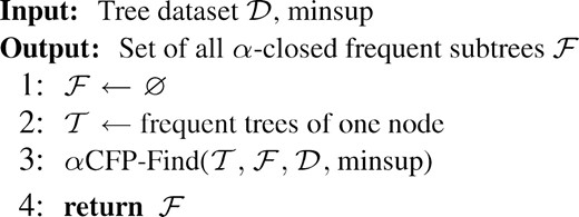
Pseudocode of main routine.

Open in new tabDownload slide

Fig. 4.

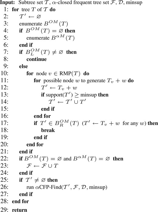
Pseudocode of subroutine αCFP−Find(𝒯,ℱ,𝒟,minsup).

Open in new tabDownload slide

2.3 Ranking frequent subtrees by statistical hypothesis testing

The frequency of each obtained α-closed frequent subtrees are not necessarily good criterion to judge the significance of the pattern, since the frequency can be simply biased by the distribution of monosaccharides. A significant pattern should be that which distinguishes given glycans from a control dataset, say randomly generated trees. Thus given a (positive) set of trees, we generate a control dataset by the following three steps: (1) We compute the distribution of parent–child pairs in the given set, (2) for each tree of the given set, we replace each parent–child pair with another one according the computed distribution, keeping the structure of the tree and (3) we repeat this procedure for all trees over the dataset. For each frequent subtree, we count the number of examples containing this pattern in the positive and the control datasets, and generate a 2 × 2 contingency table, which can be shown in Table 1. We check the independence in the contingency table by one-sided Fisher's exact test, which is exact for testing independence and can be applied to any distribution while other popular tests such as χ² test and Z test are approximations, assuming the normal distribution. Using the notations shown in Table 1, the probability that a table is generated follows hypergeometric distribution which is given as follows:

The P-value of the one-sided Fisher's exact test on a table can be computed by the sum of all probabilities of tables that are more extreme than this table.

Table 1.

Open in new tab

A 2 × 2 contingency table for a frequent pattern T

.	Positives .	Controls .	Total .
With T	# true positives (nTP)	# false positives (nFP)	n  T
Without T	false negatives (nFN)	true negatives(nTN)
Tota	n  P	n  N	n

.	Positives .	Controls .	Total .
With T	# true positives (nTP)	# false positives (nFP)	n  T
Without T	false negatives (nFN)	true negatives(nTN)
Tota	n  P	n  N	n

Table 1.

Open in new tab

A 2 × 2 contingency table for a frequent pattern T

.	Positives .	Controls .	Total .
With T	# true positives (nTP)	# false positives (nFP)	n  T
Without T	false negatives (nFN)	true negatives(nTN)
Tota	n  P	n  N	n

.	Positives .	Controls .	Total .
With T	# true positives (nTP)	# false positives (nFP)	n  T
Without T	false negatives (nFN)	true negatives(nTN)
Tota	n  P	n  N	n

We rank the obtained frequent patterns according to the P-values and if necessary choose the top patterns only. This case, given k, i.e. a prefixed number of the frequent patterns to be selected finally, we can take the following procedure: whenever each pattern is obtained in the mining procedure, we keep this pattern if its P-value is smaller than the largest one of the top k lowest P-values, otherwise it is discarded. In this manner, we can keep the necessary memory space at a fixed size, avoiding the computational load caused by taking a two-step procedure: generating all frequent patterns once and then sorting them by their P-values.

2.4 Classification with significant patterns

We here show a method of applying the obtained significant subtrees from a dataset in some glycan class to predict whether an arbitrary glycan can be in this class or not. Our idea is to generate an ensemble of classifiers, each of which is a simple classifier made by each significant pattern. Let P={P₁,…,P_|P be a set of obtained significant patterns. Let f_P(T) be a simple classifier (or a decision stump) which outputs +1 if input tree T has significant pattern P, otherwise −1 is outputted. Using f_P1(T),…,f_P|P|(T), we can generate an ensemble classifier which is weighted by w:=(w₁,w₂,…,w_|P|)′ as follows:

We can then optimize w and b of this ensemble from a given dataset of glycans with labels: {(T₁, y₁),…,(T_n, y_n)} (y_i is the label of T_i) under the criterion of maximizing the margin, which is given in the following:

where f_i :=(f_P1(T_i),…,f_P|P|(T_i))′.

We note that this manner of optimization makes our ensemble classifier equivalent to a linear support vector machine with soft margin which is so-called ν-SVM (Schölkopf and Smola, 2002). This means that from a view point of SVM, mining significant patterns is equivalent to selecting features/attributes which are significant in classification beforehand. An important, distinguished aspect of the application of our mining method to classification is that selected features are a real significant set of subtrees, meaning that we can easily show the features that work for classification in an easily comprehensive manner.

3 EXPERIMENTAL RESULTS

3.1 Mining significant subtrees

3.1.1 Data

We used all glycans in the KEGG Glycan database (Hashimoto et al., 2006). We removed entries of monosaccharides only and those containing nodes labeled by phosphorus (P) and sulfur (S). The total number of glycans we used for positives is 7454. Glycans can be classified into roughly 10 classes, according to subtrees or cores including the root. Table 2 is the list of classes and their numbers included in the data we used.

The control data we used for hypothesis testing has 7454 trees which were generated in the following manner: For each of the above 7454 positive glycans, we used the tree structure and replaced each parent–child pair of this tree with another one randomly, keeping the total distribution of parent–child pairs at the same as that of positives.

3.1.2 Mining results

Figure 5. shows the number of α-closed frequent subtrees obtained by changing α. We note that in this experiment, minsup is given by the minimum support divided by the total number of positives. This figure shows that parameter α worked well for reducing and adjusting the number of frequent subtrees. For example, when minsup was 0.5%, if α was 100%, the number of frequent subtrees was around 1500, while it was reduced to approximately 600 at α of 90% and 300 at α of 50%. We then checked only the top 10 subtrees due to space limitation. Table 3 shows the top 10 patterns with their supports and P-values, all of which were obtained by ranking according to Fisher's exact test when minsup=0.5% and α=40%.

Fig. 5.

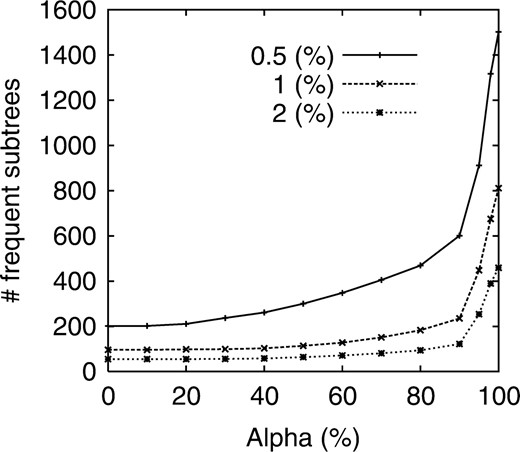
Number of frequent subtrees versus α for all glycans when minsup is 0.5%, 1% and 2%.

Open in new tabDownload slide

Table 3.

Open in new tab

Top 10 subtrees obtained when minsup = 0.5% and α=40%

Table 3.

Open in new tab

Top 10 subtrees obtained when minsup = 0.5% and α=40%

We first note that the support values of the subtrees, ranked by P-values, were not necessarily monotonically decreasing. For example, the subtree ranked at the fourth had the support of 233, which was larger than those of the second- and the third-ranked subtrees.

We emphasize that all these top ranked subtrees have biological significance individually. The first-ranked subtree is closely related with human Lewis blood group system, which categorizes humans by oligosaccharides which attached to the red blood cell membrane. These oligosaccharides are classified into roughly two types: Type 1 and Type 2. The first-ranked subtree is the common structure found in the oligosaccharides of Type 2, including Lewis X, Lewis Y and sialyl Lewis X. These oligosaccharides are biologically very important, and for example, sialyl Lewis X is expressed in a variety of cancer cells as well as the red blood cell surface and play important roles in cell–cell communications, meaning that this subtree is a key motif in glycobiology (Varki et al., 1999). We emphasize that this subtree is basically found at leaves of glycans rather than at their internal nodes. More importantly, this subtree can be found in a variety of classes, particularly glycoprotein, glycolipid and proteoglycan. We stress that it has been difficult to capture this type of motifs before our method was proposed. The second-ranked subtree is the core of a major glycan class, O-glycan, meaning that a glycan having this subtree as the core is automatically classified into O-glycan. The third- and fourth-ranked subtrees are the core of another major glycan class, Glycosphingolipid, particularly the lactoseries subclass. The fifth-ranked subtree is also related with human Lewis blood group system. This subtree is the common subtree found in the oligosaccharides of Type 1, which include Lewis A, Lewis B and sialyl Lewis A. This motif is also found in external parts of glycans throughout a lot of different glycan classes, implying that this is also an important motif in glycobiology. The sixth-ranked subtree is a core of the most major glycan class, N-glycan. Glycans in this class can be further divided into three subclasses, according to the types of internal nodes: High-mannose, complex and hybrid. The sixth-ranked subtree is the core of the high-mannose type, while the seventh-, the eighth-, and the ninth-subtrees are the core of the complex type. The N-glycan core is not only used for glycan classification but also biologically significant since it is known to be a precursor of N-glycans in synthesis and the precursor length affects the quality control of glycoprotein folding and degradation (Banerjee et al., 2007). The tenth-ranked subtree is related with human ABO blood group system. This system also uses three different types of oligosaccharides on the blood cell surface: type A, type B and type H, corresponding to group A, group B and group O. The tenth-ranked subtree is exactly the type H oligosaccharide which is known as a precursor of other two types: type A and type B. All these results indicate that our method allows to automatically capture biologically significant motifs.

3.2 Application to classification

3.2.1 Data and experimental procedure

We focused on a major class, O-glycan, because glycans of another class are easily distinguished from randomly synthesized trees (Ueda et al., 2005). We used 485 trees which were classified into O-glycan in Table 2 as positive examples, and then synthetically generated negative (control) examples in the same manner as that written in Section 3.1.1.

The experimental procedure is 10 × 10-fold cross-validation. That is, both positive and negative examples are randomly divided into ten blocks. Nine out of the 10 blocks were used for training and the remaining one was reserved for test. This was repeated 10 times by changing the test block. And finally this 10-fold cross-validation was repeated 10 times, each time using newly and randomly generated negatives. We note that in training, positives were used for mining frequent subtrees and then both positives and controls were used for hypothesis testing. The performance of our method and competing methods was measured by AUC (the area under the ROC curve) and accuracy, which was obtained by placing a cut-off value for each output at zero. The final results were averaged over 100 runs of the above cross-validation procedure. We further checked the significance of the difference between our method and another by paired t-test.

3.2.2 Competing methods

For competing methods, we used three different kernel functions for trees with ν-SVM which was also used for our method. The first kernel, which we call convolution kernel, enumerates all possible subtrees of given two trees and counts the common subtrees between the two trees (Kashima and Koyanagi, 2002). We then used a kernel, which we call co-rooted subtree kernel (Shawe-Taylor and Cristianini, 2004), uses only a part of all subtrees. The third kernel, which we call 3-mer kernel enumerates all possible subtrees with three nodes of given two trees and counts the common subtrees of them (Hizukuri et al., 2005), meaning that this kernel is also focusing on only a part of all subtrees. We note that Yamanishi et al. (2007) examined all these three types.

3.2.3 Performance results

We fixed minsup = 2 and varied α from 1 to 0.7 [We stopped there since as in Fig. 5, the number of features (subtrees) is so small when α is less then 0.7.]. Table 4 shows the AUC of the four methods and P-values (in parentheses) between our method (α=0.95) and other competing methods. Figure 6 shows the (a) AUC and (b) accuracy of our method when changing with α. Our method outperformed competing three methods, being statistically significant in all three cases, and indicating that changing α worked effectively to achieve the highest performance. We note that our method selected subtrees in terms of mining α-closed subtrees. On the other hand, the convolution kernel used simply all possible subtrees, and the rooted subtree kernel and the 3-mer kernel used only the part of them, without considering both of the frequency of subtrees in data and distinguishing positives from negatives. Thus, in this sense, this result would be reasonable. Another item of note is that our method can easily show the subtrees which work well for classification, while other three kernels cannot. We further note that the computational burden of kernel methods rises with a much higher speed as the data size increases, when compared with our method.

Fig. 6.

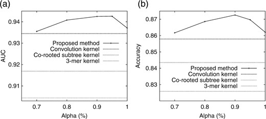
Performance results: (a) AUC and (b) Accuracy.

Open in new tabDownload slide

4 CONCLUSION AND DISCUSSION

We have presented a method for mining significant subtrees or motifs from carbohydrate sugar chains. The key contribution can be summarized in the following two: (1) We have presented a new concept in data mining, i.e. mining α-closed frequent subtrees and an efficient method for this purpose. (2) We have proposed to apply hypothesis testing to finding significant subtrees. We verified the effectiveness of our method from two different viewpoints: First, we examined the top 10 ranked subtrees at some parameter setting and found that they were all consistent with significant motifs or cores in glycobiology. Second, we applied the proposed method to a classification issue and found that our method outperformed competing methods, SVM with tree kernels, being all statistically significant.

The top 10 subtrees we checked were all known in glycobiology, but if we check subtrees ranked below the top 10 in Table 3, we might be able to find new glycan motifs which are still unknown in the literature. We emphasize that the effectiveness of our method can be clearly shown by using a large-sized dataset, such as that with a 10 000 or a million entries. In this sense, the current database is still small though increasing in a high speed. If we have a larger-sized database of glycans in the future, our method will work in many interesting issues, such as finding tree motifs which are peculiar to particular cells, e.g. cancer cells.

Funding: This work has been supported in part by BIRD of Japan Science and Technology Agency (JST), Research Fellowship for Young Scientists from Japan Society for the Promotion of Science (JSPS), and Grant-in-Aid for Young Scientists from Ministry of Education, Culture, Sports, Science and Technology (MEXT), Japan.

Conflict of Interest: none declared.

REFERENCES

Author notes