


Abstract
Motivation: Some functionally important protein residues are easily detected since they correspond to conserved columns in a multiple sequence alignment (MSA). However important residues may also mutate, with compensatory mutations occurring elsewhere in the protein, which serve to preserve or restore functionality. It is difficult to distinguish these co-evolving sites from other non-conserved sites.
Results: We used Mutual Information (MI) to identify co-evolving positions. Using in silico evolved MSAs, we examined the effects of the number of sequences, the size of amino acid alphabet and the mutation rate on two sources of background MI: finite sample size effects and phylogenetic influence. We then assessed the performance of various normalizations of MI in enhancing detection of co-evolving positions and found that normalization by the pair entropy was optimal. Real protein alignments were analyzed and co-evolving isolated pairs were often found to be in contact with each other.
Availability: All data and program files can be found at Author Webpage
Contact: [email protected]
Supplementary information: Author Webpage
1 INTRODUCTION
Multiple sequence alignments (MSAs) of homologous proteins carry evolutionary information. Changes due to the mutation of amino acids at various positions in a protein are passed on to the next generation and may therefore reappear, through speciation, in the proteins of closely related organisms. In many instances functionality imposes constraints on these mutations, and important amino acid positions are often conserved. However mutation studies have shown that many non-conserved positions may also be functionally important. In particular, there may be compensatory mutations such that a mutation in one column of the MSA is typically matched by a corresponding mutation in another column. These co-evolving mutations are of key interest as they may identify residues that interact within the protein, residues which are functionally or structurally important, or possibly key sites of interaction between the protein and its substrate.
Mutual information (MI) is a measure of reduction of uncertainty (Ash, 1965; Cover and Thomas, 1991). In an MSA, the MI between two positions (columns) reflects the extent to which knowledge of the amino acid at one position allows us to predict the identity of the amino acid at the other position. MI values are high if substitutions at the two positions are correlated. MI is thus a natural measure with which to identify sites of correlated and compensatory mutations in homologous proteins.
Many investigators have reasoned that co-evolving positions in sequence alignments must be correlated and thus identifiable. Such identification is difficult because the signal that occurs due to compensatory mutations must be separated from the background signals that occur because of phylogenetic influences and small sample size effects (Atchley, 2000). Oliviera et al. (2002) developed a qualitative method, Correlated Mutation Analysis (CMA), to identify co-evolving residues based on the variability, entropy and correlation of the residues. However, their method determines important sites using a moving cutoff that differs with every protein family. Singer et al. (2002), in a variation of CMA using empirically derived likelihood scores, predicted residues to be in contact with a 16% accuracy for a variety of protein families. Pritchard et al. (2001) used the number of branching events for each residue to identify co-evolving sites. In previous studies that used MI, Korber et al. (1993) compared MI from an MSA to that from multiple randomizations of the original MSA and identified strongly co-varying residue pairs. Clarke (1995) corrected MI values by a metric corresponding to the number of observed amino acid pairs at each position. Wollenberg and Atchley (2000) used a model of phylogenetic substitution to attempt to correct for this background. However, most of these studies focused on those residue pairs with the highest MI values and assigned only qualitative significance to their scores. Tillier and Liu (2003) used mutual information and mutual interdependence to identify positions that co-evolved with each other, but were not co-evolving significantly with other positions in the alignment. Their method was highly selective, and did not rely on knowing the underlying relationships between the sequences, but could potentially miss positions that co-evolved with several others. As yet, no single method has demonstrated general utility or achieved widespread acceptance.
Here we review the mathematical underpinnings of MI and its application to MSAs. Using simulated MSAs we quantify the background levels of MI due to the limited numbers of sequences and the underlying mutation rates; we then use in silico evolution to examine the contribution of shared evolutionary history. To simulate co-evolution due to structure or function, some positions are constrained to mutate in concert; the effects of these constraints are analyzed by comparing the MI of such pairs with the distribution of the MI of all position pairs in the alignment. In this comparison, the unconstrained positions provide a distribution of background signals arising from the phylogenetic relationships among the sequences and their limited number, sources common to all position pairs. A number of normalizations were tested for enhancement of the co-evolutionary signals above the background in the simulated sequences; division of MI by the pair entropy, a mathematically justifiable normalization, was optimal. This normalization was then applied to real protein MSAs, allowing us to identify position pairs that usually make contact in 3D protein structures.
2 MUTUAL INFORMATION
MI is a well known measure in Information Theory. Motivations for its properties and an axiomatic derivation are given by Ash (1965) and complementary material is found in Cover and Thomas (1991). We first give an overview of MI and then describe how it is applied to an MSA.
2.1 Definition and formulation of MI
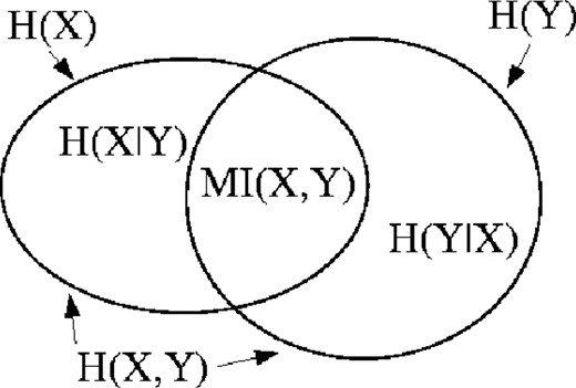
Venn diagram of entropy space.
2.2 Mutual Information applied to MSAs
In an MSA, the amino acids in a given column can be considered as a set of observations of a random variable x. An estimate of the entropy H(X) is obtained by using the observed amino acid frequencies, f(xi), in place of the underlying probabilities, p(xi), in Equation (1). A similar estimate for H(X, Y) can be made using a second column in the MSA and the frequencies of all ordered pairs (xi, yj) occurring in the rows of the two columns. It is then straightforward to obtain an estimate of MI(X, Y) for that pair of columns by applying Equation (5).
The MI between two columns reflects the degree to which the pattern in the two columns is correlated. If amino acids occur independently at the two sites, the theoretical value for MI is zero. However, the estimate of the MI will only be zero if the observed pair frequencies reflect all possible pairings for the observed amino acid frequencies. Such a case is illustrated in Figure 10e, where X = {A, C; f(A) = 1/3, f(C) = 2/3} and Y = {E, M; f(E) = 1/2, f(M) = 1/2}. Adding or deleting a row would result in different pair frequencies and yield a non-zero value of MI(X, Y), as would interchanging dissimilar amino acids within a column.
When considering independent columns within finite MSAs, those alignments with fortuitous pairings resulting in vanishing MI values are the exception, as any deviation from the ‘all possible pairs’ representation will yield a positive MI value. Also, as the number of amino acids occurring increases, the minimum sample size for which zero MI is possible increases quickly. If all 20 amino acids are present in each column and are equally probable, then zero MI is only possible if the frequency of each pair of amino acids is 1/202. This condition cannot be met in an MSA with <400 homologous proteins, and is unlikely to be met in columns of finite length. A statistical interpretation of MI is discussed in Cline et al. (2002), along with some cautionary remarks on the sample size.
3 SIMULATED MSAs
To investigate the properties of MI when applied to MSAs, we generated and analyzed simulated data. Although we recognize that in silico evolved sequences are unable to mimic many of the salient features of real MSAs, this process allowed us to isolate the effects of a number of key parameters on background MI. In particular, we examined the variation of MI with the number of sequences in the alignment, the size of the amino acid alphabet and the mutation rate used to generate the MSA. All parameters impact the mean entropy of the aligned columns, which is the measurable characteristic for MSAs obtained from real proteins. We first simulated MSAs in which mutations at each position in the protein were completely independent. This allowed us to quantify background MI. We then introduced co-evolving sites and evaluated the performance of MI in finding those sites. We expect that any correlated substitutions will have an observed MI above background values.
3.1 Background MI
There are two sources of background MI: finite sample size effects and phylogenetic influence.
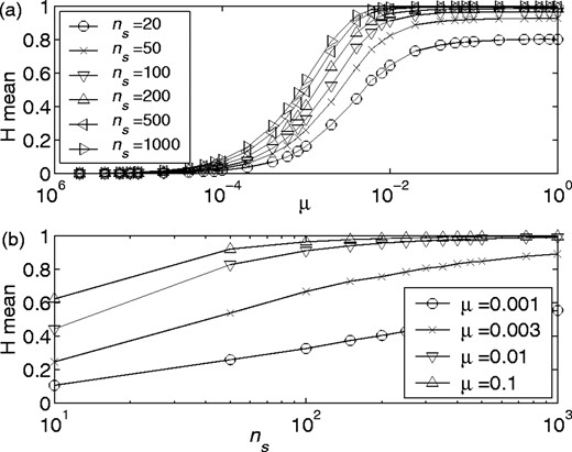
Finite sampling effects. To quantify the effects of finite sample size on MI, we produced simulated MSAs in two ways. We produced matrices of ns rows (sequences) and nr columns (residues). Initially, all the entries were identical. Each position in the matrix was then allowed to ‘mutate’ with probability u. If a mutation occurred, one of na (alphabet size) amino acids was randomly selected to replace the existing one. In the first case all members of the alphabet were equally probable. We then repeated this process, but selected the amino acid introduced by the mutation by using frequencies of amino acids observed in MSAs from real proteins. In particular, each column was randomly assigned to have the amino acid frequencies from one of the 314 ungapped columns of the MSAs for ATP synthase epsilon and gamma subunits (see the website for MSAs). Figure 2 shows the rapid decrease in mean MI as the number of sequences in these randomly generated alignments increases for either scenario. We note that alignments with amino acid frequencies from real proteins carry significantly less background MI on average. This is presumably because a number of columns are somewhat conserved and so have low entropies. Recall that the minimum entropy of either column is the maximum value that the MI can attain. Figure 2 suggests that for realistic amino acid frequencies, the contribution of background MI from finite column lengths is not too severe (when compared with values typically found in real protein alignments, see for example Fig. 9), particularly when the number of sequences in the alignment is greater than ∼150.

Mean background MI versus the number of sequences for ‘non-evolved’ sequences with various mutation probabilities u: mutations to each amino acid equiprobable (a) and amino acid substitution probabilities based on the frequency of amino acid occurrence in ATP synthase (b). A total of 1000 pairs of columns were randomly generated for each data point. Note that a value of 20 is used as the logarithm base (b), and the maximum MI attainable is 1.
Phylogenetic influence. The second source of background MI is the evolutionary past inherent in every MSA of homologous proteins. In biologically meaningful alignments, no two positions can be independent, since two residues in the same protein are generally inherited as a unit. Thus, even when substitutions at the two sites occur with complete independence, the shared evolutionary history contributes a large background to the measured MI between those positions.
We quantified this effect by creating MSAs through in silico evolution. Binary trees with ns tips were evolved using an initial sequence of identical amino acids, a branching probability pb, a site mutation probability μ and equiprobable amino acid substitution. Sequences at the tips of the branches were then collected to form the simulated MSA.
Note that the ‘timestep’ used in this simulation is arbitrary, since both μ and pb are probabilities per timestep. The important non-dimensional parameter is the ratio of μ to pb, which gives the average number of substitutions between branch nodes. Thus arbitrary values of μ and pb will give equivalent results, as long as this ratio is maintained. A value of pb = 0.01 was used in all the simulations.
This simple evolutionary model gives higher background levels of MI than other more complex models of evolution, thus providing a stringent test of our ability to detect co-evolution. MSAs evolved using a variety of more complex models from the PAML package (Author Webpage) exhibited background MI with the same behavior though slightly reduced in magnitude (Supplementary data are shown at Author Webpage).
An MSA of real proteins typically represents a small sample of branch tips from a much larger evolutionary tree. We might therefore simulate a very large binary tree and then randomly eliminate branches until ns ‘species’ remain in the simulated MSA. This strategy is, however, formally equivalent to the technique described above, which simulates only the species that are ultimately part of the MSA. It should be noted that real MSAs do not meet this ideal of random sampling. In general, there are many examples of sequences from closely related sequences (e.g. pathogens). Finally, although it may be extremely difficult to estimate μ/pb from a real MSA of homologous proteins, we are fortunate in that the mean entropy of the columns in the MSA grows monotonically with mutation rate (Fig. 3). Thus to simulate data that are analogous to a given real MSA of length ns, we can choose an arbitrary branching ratio pb, and then find the value of μ that gives an entropy similar to that of the real data.
Mean column entropy versus mutation rate (a), and number of sequences (b), for in silico evolved MSAs. Both plots are for amino acids alphabet size of 20 (na) and for sequences 100 residues in length (nr). A binary tree branching probability of 0.01 (pb) was used to evolve the sequences. Each data point is the average of values from 50 MSAs.
Combined effects. This framework allows us to quantify the combined contribution of finite sequence lengths and shared evolutionary history to background MI. Figure 4 plots the mean background MI versus the number of sequences in an alignment; the figure is analogous to Figure 2, but for sequences evolved in silico as described above. Once again, we have not included any correlated substitutions in the simulated MSA, and therefore we might expect that the MI should be close to zero. However Figure 4 shows significant background MI due to the inherent correlations in sequences that share an evolutionary history. Figure 4a shows the decline in background MI as we add more sequences to the alignment; to generate these data μ/pb was held fixed at 0.1, and the alphabet size was adjusted to investigate various possible interpretations of an MSA. These values are na = 2 (of theoretical interest), 4 bases, 20 amino acids or 64 codons. In the second panel, we held na fixed at 20 and varied μ. This dataset demonstrates that for very low values of μ/pb, the background MI contributed by shared evolutionary history is small, but is still increasing even when we have 1000 sequences in the alignment.
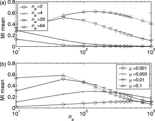
Mean background MI versus number of sequences, ns, for various ‘amino acid’ alphabet sizes, na (mutation rate held constant at μ = 0.01) (a), and for various mutation rates, μ (amino alphabet size held constant at na = 20) (b) for in silico evolved MSAs (pb = 0.01). The logarithm base is set to the alphabet size (i.e. b = na) in the calculation of MI values. Both plots are for sequences 100 residues in length (nr). Each data point is the average of values from 50 MSAs.
Figure 5 offers two additional views of the multi-dimensional relationship between background MI and the parameters ns and μ/pb. In Figure 5a background MI is plotted against μ for various MSA lengths. We can see that MI generally increases with higher mutation rate, rising rapidly to a plateau value. With large numbers of sequences in the alignment, MI may exhibit a peak before plateauing at a lower level. Some intuition can be gained by noting that the worst case for finite sampling effects (i.e. the longest alphabet and smallest number of sequences) in this dataset, ns = 20, has the highest plateau. As stated previously, the ideal case of zero background MI cannot be realized with short columns, but is approached more closely as ns increases. Thus plateau levels are lower for alignments with more sequences.
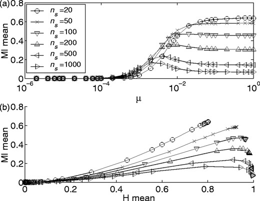
Mean background MI versus mutation rate (a), and mean entropy (b). Both plots are for na = 20, nr = 100 and pb = 0.01. Each data point is the average of values from 50 MSAs.
Finally, in Figure 5b we plot the mean background MI versus the mean column entropy since this value is accessible when working with real MSAs, whereas the mutation rate is unknown. From this figure we can estimate the expected magnitude of the background MI for a given MSA with known mean entropy and ns.
3.2 Simulated MSAs with correlated mutations
We also evolved MSAs with a known dependence between some of the columns; in this evolutionary framework half the sequence is ‘partnered’ to force co-evolution between pairs of columns, and half remain unconstrained. We choose nr = 100 (a realistic order of magnitude for protein sequence length) and ns = 100 (for which there is significant background MI), and impose the constraint that for half of the positions, if one position undergoes a mutation then so does a partner. Thus positions 1 through 50 are allowed to mutate freely during evolution. Positions 51 through 75 also mutate freely but if a mutation occurs at position 51, for example, then position 76, its ‘partner’, is mutated as well, though not necessarily to the same amino acid.
With equiprobable amino acid substitution, there is a small chance that an amino acid may mutate to itself. It is also possible that it may mutate back to an amino acid that has already occurred at this position in the simulated evolutionary history. For the partnered columns, both of these effects allow for less than perfect dependence, and diminish the signal of co-evolution thus increasing the difficulty of the detection of partnered columns a posteriori. Datasets thus generated provide a test case for methods of detecting co-evolving residues.
3.2.1 Normalization
We first compare the MI for every possible pair of columns in our in silico evolved data, as shown in Figure 6 [because of symmetry, only M(X, Y) for Y > X is reported], thus determining whether the MI of partnered columns (shown as filled circles in this figure) is significantly higher than average. We see that this is not the case for a significant number of the partnered sites. The problem with this approach stems from the fact that the upper bound on MI for a given pair of columns is the lesser of the entropies of either column. Even though the partnered columns have an MI closer to saturation (45 degree line in Fig. 7a) for a given minimum column entropy than other independent columns with similar minimum entropies, the wide range of entropies present in the MSA is such that the level of background MI values due to the more entropic columns (portion of the cloud to the right) often surpasses the MI of the less entropic partnered columns. We observe that the background MI is highly correlated with the minimum entropy suggesting that normalizing MI(X, Y) by min{H(X), H(Y)} would ‘level the playing field’ and improve detection of those partnered columns with at least one low column entropy. This is true, as can be seen in Figure 7b, which shows MI/min{H(X), H(Y)} values; here the signal from the partnered sites is clearly stronger than the background. We can show, however, that detection ability may be further enhanced if we normalize by the upper bound on the MI, H(X, Y). Even though the background MI is less correlated to this quantity (Fig. 7c), the separation of the MI for partnered columns from that of background H(X, Y) peers is greater. This is demonstrated in Figure 7d, where we see that a greater fraction of the partnered sites have normalized MI values surpassing 4 standard deviations.
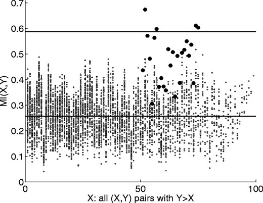
MI for all column pairs for an in silico evolved MSA (μ = 0.002, pb = 0.01, nr = 100, ns = 100, na = 20) with correlated mutations. The 25 partnered residues pairs are shown as filled circles. The average MI and a 4 standard deviation cutoff are shown as horizontal lines.
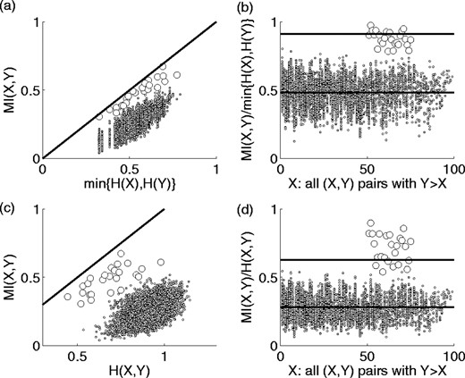
Scatter plot showing the correlation of MI with minimum column entropy for all column pairs and (45 degree) saturation line, MI(X, Y) = min{H(X), H(Y)} (a), and the effect of normalizing MI by minimum column entropy (b), both for the same data shown in Figure 6. The average MI and four standard deviation cutoff values are shown as horizontal lines. Panels (c) and (d) are similar plots for pair entropy correlation and normalization. Values for the 25 partnered pairs of residues are indicated as open circles.
For a complete analysis, we normalized MI by all possible terms (or reasonable combinations of terms) appearing in Equations (3)–(5) and tested each normalization. Each set of scores was then converted to Z scores (i.e. number of standard deviations from the mean) and column pairs that scored above an assigned Z cuttoff were identified. Sensitivity (ratio of true positives to true positives plus false negatives) and specificity (ratio of true positives to true positives plus false positives) were then calculated.
We tested normalizing MI(X, Y) by each of the following: H(X, Y), (H(X) + H(Y)), min{H(X), H(Y)}, max{H(X), H(Y)}, min{H(X|Y), H(Y|X)} and max{H(X|Y), H(Y|X)}. Normalizations MI(X, Y)/H(X, Y) and MI(X, Y)/(H(X) + H(Y)) are not independent; the distributions for each differ but the rank ordering of all MI scores remains invariant. However, since a Z-score cutoff, and not a percentile cutoff, is a more practical guideline for detecting significant sites in real proteins, we tested both.
The results of these tests for a Z = 4 cutoff are shown in Figure 8. Though most normalizations perform nearly equally well in terms of specificity, MI/H(X, Y) is demonstrably better with respect to sensitivity. Both measures are optimized for values of μ > 10−3, which in turn corresponds (viz. Fig. 3a) to a mean entropy of ∼0.3 for alignments whose size is on the order of ns = 100. Therefore these tests suggest a natural entropy cutoff when analyzing real protein MSAs. Note that in both instances, raw MI performed significantly less well than any normalization in its ability to detect partners and filter out false positives.
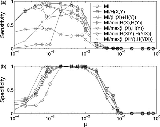
Sensitivity (a) and Specificity (b), as defined in text versus mutation rate for in silico evolved sequences. A binary tree branching probability of 0.01 (pb) was used to evolve the sequences. Various normalizations are plotted for a Z = 4 cutoff. Parameters values were the same as described in Figure 6, and data were averaged over 50 MSAs for each value of μ.
4 ANALYSIS OF REAL PROTEIN FAMILIES
In this section, we apply normalized MI to real protein MSAs. We begin by describing a representative example, and then outline two different analyses that were performed to assess the predictive power of MI and its various normalizations with respect to residue contact.
4.1 Isolated pairs in triosephosphate isomerase
A multiple sequence alignment for triosephosphate isomerase was generated as described (Cover and Thomas, 1991). Mutual information and Z scores were calculated as for the simulated alignments. Residues having an entropy >0.3 were then selected for the analysis that follows. This entropy cutoff restricted the analysis to those positions that contained sufficient variability that they were unlikely to show significant MI due to genetic linkage. One could also argue that those residues with entropy <0.3 are readily identifiable as (nearly) conserved columns. Residues that scored high in normalized MI relative to their peers (Z > 4) were identified and found to fall into two groups. The first was composed of residues that scored highly with one, and only one, other residue. We will call these ‘isolated pairs’. Isolated pairs often rank amongst the highest in the normalized MI distributions. The second group is composed of residues that score highly with more than one other residue and so form a network. Outliers belonging to this group have been determined to often be located at or near functional sites [they are discussed in detail in Gloor et al. (2005) and will not be further discussed here]. We now give an example illustrating the effect of normalization on those residues that are later identified as isolated pairs.
In Figure 9 we show MI and normalized MI for all pairs above the 0.3 entropy cutoff in the TIM alignment. In each plot, the data points for the isolated pairs are shown as open circles. One pair is nearly an outlier with respect to the MI distribution, and has the second-highest MI score. The other two pairs rank much lower and are at MI levels met by a significant portion of the cloud. After normalization, these three pairs have the highest Z scores in the entire alignment (5.9, 4.4, 4.1). The three column pairs, (184,227), (68,70) and (135,176), were also the only outliers for this protein and were each singly connected, or isolated, pairs. The minimum separation between non-hydrogen atoms of these residues in the X-ray structure 1IIH.PDB (Noble et al., 1991) are 3.0, 3.5 and 7.6 Å.
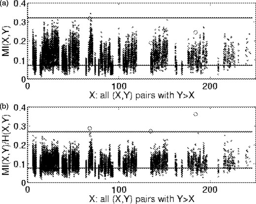
MI (a) and normalized MI (b) versus position for triosephosphate isomerase. Horizontal lines are mean values (lower) and Z = 4 cutoff values (upper) for each case. Open circles are isolated pairs.
4.2 Larger datasets—distant residue contact
Multiple sequence alignments for the Conserved Domain Database (CDD) (Marchler-Bauer et al., 2005) were obtained from the NCBI (January 2005) and used for the analysis. Alignments for protein families from PFAM (Alex et al., 2004), COG (Tatusov et al., 2003) and CDD were extracted from this dataset if they included one or more structures and contained at least 30 sequences. The 941 resulting alignments were examined for the presence of poorly aligned members. Sequences were removed from the alignments if they had 20% or more gaps than the reference structure's sequence. Applying this rule resulted in 616 suitable sequence families. The MI and Z score for each pair of residues in the 616 protein families above the 0.3 entropy cutoff was determined as for the modeled alignments. Seventy-five percent of these families (464 of 616) had one or more residue pairs with a Z score >4 (‘high-scoring pairs’). This yield is substantially below that seen with alignments generated manually, where 22 of 23 alignments yielded one or more high scoring residue pairs (Gloor et al., 2005). Thus, the alignments from the domain databases are generally suitable for this analysis, but increased sensitivity can be achieved by careful editing of the alignments.
We used these alignments to test the same hypothesis that was tested in Section 4.1 (that isolated pairs should be close in 3D space), but we added the constraint that they should be separated by at least 10 residues in the reference sequence. Poon and Chao (2005) have shown experimentally that co-evolving residues are often in physical proximity, and this measure was also used by Tillier and Liu (2003) to test their ability to find co-evolving positions. For this, we measured the distance between positions in the 361 alignments (142 COG, 95 PFAM and 124 CDD alignments) that contained at least one isolated pair separated by 10 or more residues in sequence. The data in the first row of Table 1 show that the mean distance between the 435 isolated pairs in the complete set of 361 protein families is 17.4 Å compared with the average inter-residue distance of 23.0 Å in these protein families.
The mean distance between residue pairs that have Z scores of 4 or more is strongly dependent on the number of sequences in the alignments, and is independent of the separation of these residues in the primary sequence.
| Number of sequences in alignment | Mean distance (Å) | Num. of isolated pairs | Mean separation (residues) | Fraction of pairs in contact | P-value |
|---|---|---|---|---|---|
| 8–1436 | 17.4 | 435 | 98.6 | 0.26 | <1E−6 |
| >150 | 6.9 | 32 | 54.5 | 0.66 | <1E−6 |
| 125–149 | 6.6 | 15 | 52.1 | 0.47 | <1E–6 |
| 100–124 | 12.5 | 15 | 75.1 | 0.33 | 4.6E–5 |
| 75–99 | 10.4 | 40 | 80.1 | 0.48 | <1E–6 |
| 50–74 | 18.8 | 101 | 120.0 | 0.24 | <1E–6 |
| 25–49 | 18.4 | 171 | 96.5 | 0.20 | <1E–6 |
| 8–24 | 26.3 | 61 | 121.7 | 0.07 | 0.45 |
The P-value was determined by the bootstrap analysis as described in the text, and represents the likelihood of selecting the number of residue pairs in the column from the total set of all inter-residue distances, with an average inter-residue distance equal to or less than that observed. Note that all the residue pairs used in this analysis are separated by 10 or more intervening amino acids. Details may be found at Author Webpage
The significance of this difference was tested by randomly selecting with replacement, for each isolated pair, amongst those pairs from the data with the same sequence separation (bootstrap sampling). For example, for the complete dataset, 435 random inter-residue distances were selected such that the randomly selected set had the same sequence separations as the real dataset. This sampling was repeated for 106 trials. The proportion of the trials that had a mean distance of 17.4 Å or less was then reported. We observed that none of the 106 random samples had a mean distance of 17.3 Å or less (i.e. P < 106), and thus conclude that it was extremely unlikely to choose a set of 435 inter-residue distances with this mean distance from the set of residue pairs with the same sequence separations by chance. This was done for datasets of MSAs with varying number of sequences and the results are shown in Table 1. All but the smallest MSA sets (8–24 sequences) have isolated pairs whose average distance is significantly less than that expected by chance.
Our modeled data also indicated that there should be a strong relationship between the specificity of the method and the number of sequences in the alignment. We therefore stratified the data and found that the high-scoring residue pairs from the 36 alignments containing at least 125 sequences were separated by <7 Å on average, but had a mean sequence separation of over 50 residues. Almost 60% of these residues were in contact (28/47, defined as a side-chain separation of 5 Å or less in the representative structure). In contrast, the mean distance for residue pairs from the alignments containing <125 sequences was at least 11 Å, and generally <30% of these were in contact. Therefore, the number of sequences in the alignments is a critical parameter for the detection of such positions, and we conclude that the modeled data accurately represent the minimum number of sequences required to extract useful MI values from real alignments.
4.3 Maximum residue MI
As described above, the various normalizations changed both the absolute value of MI and the rank order of pairs. To focus on the effects of the latter in our ability to detect pair contact, we examined the relationship between the maximum score achieved by a residue under the various normalizations, and the distance between the residue and its MI partner in the 83 alignments containing at least 125 sequences. Note that we are no longer restricting our analysis to isolated pairs. As before, this analysis was restricted to residues with entropies of 0.3 or greater and residue pairs separated by 10 or more other residues in the reference sequence.
This set of MSAs provided 1 097 964 residue pairs of which 23 612 (or 2.2%) were in contact (a side chain separation of 5 Å or less). The number of residue positions that met the entropy cutoff constraint was 8556. The number of contacts identified by each normalization is given in Table 2. We observe that maximum MI without any normalization identifies the least number of contacts, whereas there is a significant improvement in accuracy when maximum conditional entropy, maximum entropy, sum of entropies and pair entropy are each used to normalize MI. Pair entropy and sum of entropies identified the greatest number of contacting residues, albeit by a small margin over the previous two, and identified 46% more than un-normalized MI.
Number of residue positions, X, whose maximum MI(X, Y) for all Y that are separated by 10 or more amino acids successfully predict side chain contact with Y.
| Normalization | Number of maxima in contact | Fraction of maxima in contact (%) |
|---|---|---|
| 1 | 840 | 9.8 |
| min{H(X|Y), H(Y|X)} | 877 | 10.3 |
| min{H(X), H(Y)} | 877 | 10.3 |
| max{H(X|Y), H(Y|X)} | 1218 | 14.2 |
| max{H(X), H(Y)} | 1218 | 14.2 |
| H(X) + H(Y) | 1228 | 14.4 |
| H(X, Y) | 1228 | 14.4 |
All normalizations are tested and results are expressed both as a number and as a fraction of eligible (X, Y) pairs.
Some of the table entries are identical. As noted earlier, normalization by H(X) + H(Y) is not independent from H(X, Y) normalization, and so we obtain the same rank ordering in the transformations induced by these normalizations. Normalization by minimum entropy or conditional entropy yields the same highest scoring pair since, upon rewriting Equation (3) as H(X|Y) = H(X) − MI(X, Y) along with H(Y|X) = H(Y) − MI(X, Y), we can see that for a given MI(X, Y), finding the maximum entropy of X or Y is equivalent to finding the corresponding conditional entropy.
To reiterate, by exclusively considering the highest MI and normalized MI values for each residue position, we do not rely on the form of the underlying distributions, nor on a cutoff (i.e. 4Z or 4 standard deviations from the distribution mean, the value of which requires guidance from the analysis of simulated evolutions). We have shown that the rank ordering induced by pair normalization yields top scoring pairs that are more frequently in contact than those of other normalizations.
5 DISCUSSION
5.1 The effect of normalizing MI by H(X, Y)
To clarify the effect of the normalization that we propose, it may be useful to consider several hypothetical MSAs and their corresponding Venn diagrams, as illustrated in Figure 10. In cases (a) and (b), the H(X) and H(Y) spaces overlap exactly (see Fig. 1 for labeling). This corresponds to two columns whose elements are uniquely paired, that is, an ‘A’ in column 1 occurs if and only if an ‘E’ occurs in column 2, etc. Although only unique pairs occur in both cases, in (b) greater column entropy results in greater MI. Normalization eliminates the influence of this disparity in entropy.

Examples illustrating the effect of normalizing MI by pair entropy for MSAs with varied column entropies (area of circles) and dependencies (area of overlap). Completely dependent columns do not gain by an increase in entropy (a versus b) with normalized MI. Similarly, columns with a similar amount of unnormalized MI rank lower in normalized MI (c versus d) if the overall entropy of the columns is greater.
In case (c), the pairings are not unique; in particular an ‘E’ might correspond to either an ‘A’ or a ‘C’. Here the uncorrected MI is similar to that in case (a), but when normalized there is a penalty associated with non-uniqueness. Likewise case (d) illustrates non-uniqueness in both directions. Because of the high column entropy the MI is large. Again, normalization reduces this effect. Case (e) demonstrates that when all possible ordered pairs occur at frequencies expected for two independent columns, both MI and normalized MI are zero.
When applied to MI from MSAs, the H(X, Y) normalization ranks the column pairs in the order of most unique mutations. For real protein evolution there may be subsets of the amino acids that are equally viable as compensatory mutation residues, several of which would appear in different homologous proteins. Those co-evolving sites would not score as well under this normalization.
6 CONCLUSIONS
We have investigated the properties of MI when applied to MSAs. In particular, we have quantified two sources of background MI for uncorrelated sites: finite sequence sampling effects and phylogenetic influences. Quantifying sampling effects suggests that background MI is a significant obstacle for alignments that have <125–150 sequences. A significant amount of background MI is due to the phylogenetic fingerprint on an MSA, even when mutations occur independently.
Evolution of MSAs via in silico evolution was carried out with a very weak set of rules for co-evolution, specifically no restrictions were placed either on the amino acid identity for mutations or on that of compensatory mutations when partnered sites mutated. We found that normalizing MI by the pair entropy optimized the ability to detect co-evolving sites over a large range of mutation rates. Importantly, our method requires no assumptions about either the underlying relationships between the proteins in the alignment or how rapidly or slowly the sequences may be evolving. The method only assumes that the MI caused by shared inheritance is relatively constant across each sequence, and that most pairs do not share significant MI due to structural or functional constraints. The significance scores thus reflect how much more MI a given residue has than its peers in that alignment.
We have applied this measure to MSAs obtained from real protein alignments and found that normalization notably improved the identification of important residue pairs that are in contact in the folded structures of the protein; most of the co-evolving, isolated pairs are in contact with their partner in representative structures. These residues may prove important to the structural stability of the folded protein.
This work was supported by the Natural Sciences and Engineering Research Council of Canada, Canadian Institutes of Health Research and the Ontario Ministry of Science, Technology and Industry (Premier's Research Excellence Awards). Funding to pay the Open Access publication charges for this article was provided by the University of Western Ontario.
Conflict of Interest: none declared.

