


Abstract
Co-fractionation mass spectrometry (CFMS) enables the discovery of protein complexes and the systems-level analysis of multimer dynamics that facilitate responses to environmental and developmental conditions. A major challenge in CFMS data analysis, and omics approaches in general, is the development of reliable benchmarks for accurate evaluation of prediction methods. CORUM is commonly used as a source of benchmark complexes for protein complex composition predictions; however, its assumption of fully assembled subunit pools often conflicts with size exclusion chromatography (SEC) and interaction predictions from CFMS experiments. To address this, we developed an integrative analysis method that leverages cross-kingdom evolutionary conservation among specific CORUM complexes and high-resolution SEC profile data from cell extracts. The resulting benchmark complexes are supported by statistical significance and consistent sizes between calculated and measured apparent masses. The approach was robust, revealing both conserved and species-specific complexes. Designed specifically for benchmark identification, this method can be applied to any species and used to evaluate protein complex predictions from other studies.
Introduction
Co-fractionation mass spectrometry (CFMS) is a high-throughput, mass spectrometry-based protein quantification method coupled with biochemical fractionation to analyze protein complex compositions under non-denaturing conditions. This “guilt by association” method was initially used to predict protein organelle localization based on co-elution with known marker proteins [1] and was subsequently applied to predict protein interactions [2, 3]. The technique evolved from the principle that proteins present in a stable complex co-migrate independent of the separation method used. In life sciences, CFMS has been extensively employed to analyze protein complex dynamics, including protein–ligand interactions, circadian changes, and multimerization variants across various species and tissues [4–10]. However, a universal major challenge lies in evaluating CFMS-based predictions due to the lack of reliable benchmarks [11, 12]. Protein complex predictions rely on known protein complexes from reference databases, such as the CORUM mammalian protein complex database [13] as benchmark data. Reliable benchmarks are crucial for defining accuracy measures, such as precision and recall, in protein complex predictions. Inaccurate benchmark data result in flawed validation datasets, which in turn mislead prediction models to unreliable predictions.
Ortholog mapping revealed that a substantial number of CORUM complexes are highly conserved across animals and plants (see the Results section). This conservation is expected, as many of these complexes perform essential functions in eukaryotic cells. For example, very similar protein complexes are involved in processes such as DNA replication, gene expression, vesicle trafficking, signal transduction, and metabolism in eukaryotic cells [14]. Orthologs of CORUM complex subunits can be accurately identified across species using tools such as InParanoid [15] or EggNOG [9, 16–18]. Most CORUM complexes were derived from highly purified multimers and used to generate solved crystal structures [19–24]. However, this does not mean that the fully assembled state is the major protein pool in cell extracts. They may primarily exist as partially assembled complexes or CORUM subunits interacting with unknown proteins as part of a “moonlighting” function [25].
CORUM complexes are widely used as benchmarks for evaluating protein complex predictions. During evaluation, pairs of subunits in the reference CORUM complexes are assumed to comprise a positive set of protein–protein interactions, while negative interactions are created from proteins not present in the positive interaction set. These positive and negative sets have been used for training and testing computational methods of protein complex predictions [9, 12, 18, 26], inherently assuming that CORUM complexes exist in a fully assembled state. However, our previous work employing size exclusion chromatography (SEC) profiling of CORUM subunits revealed widespread violations of this assumption [6, 27]. Furthermore, recent publications related to animal cell extracts have also reported weak correlations among subunits of CORUM complexes in the CFMS datasets [12, 18]. Pang et al. [12] displayed probability density plots of the Pearson correlations between fractionation profiles of shared subunits of CORUM human complexes (Fig. 2 in [12]), in which the density plots have a mode around zero correlation values. Similarly, Wan et al. [18] reported low correlation among subunits of CORUM complexes in their Extended Data, (Fig. 2 in [18]). These plots, along with our published experimental data, indicate that the most abundant cellular pools of CORUM complex subunits, which are primarily detected in liquid chromatography mass spectrometry, do not always co-elute. This suggests that CORUM complexes are unlikely to be reliable benchmarks for protein complex predictions.
Here, we implement a machine learning method that integrates two sources of information to define reliable protein complex benchmarks: evolutionary conservation from CORUM and co-elution patterns from CFMS data obtained on analytical SEC columns. We first map plant orthologs to CORUM protein complexes and then analyze their CFMS elution profiles. Subcomplex predictions are generated using self-organizing maps (SOMs) [28], a robust unsupervised learning method, and are further refined through statistical testing and mass comparisons.
To generate reliable protein complex benchmarks, we refine CORUM complexes by integrating their subunit composition with CFMS co-elution patterns. Our method eliminates random co-elution by ensuring that only subunits within the same CORUM complex are considered. We then detect subcomplexes, identifying subsets of CORUM complexes that exhibit strong similarity based on CFMS co-elution. This approach is justified by the premise that functionally related subunits tend to co-occur within stable subcomplexes, even if chance co-elution exists in the overall CFMS data. By incorporating both CORUM composition and CFMS patterns, our method refines CORUM complexes to better reflect their assembly state in cell extracts and improves benchmarking for protein complex predictions. We demonstrate the generalizability of this method through its application to rice and Arabidopsis.
Materials and methods
SEC data acquisition and filtering
We used a previously published rice SEC profiling dataset for protein complex predictions [10]. The chromatography conditions are robust [4, 6, 27] and this particular dataset contains two replicates of SEC fraction profiles along with protein apparent mass (Mapp), monomeric mass (Mmono), and multimerization state (Rapp), which is defined as the ratio of Mapp to Mmono and serves as a multimerization predictor [4, 29]. Here, Mapp represents the measured protein mass from SEC experiments. To ensure reliable protein profiles, we applied established data filtering criteria [10, 17, 27]. Reproducible protein profiles were selected if their elution peaks between two replicates fell within two SEC fractions, a threshold met by 90% of peaks. If a reproducible peak was located in the first (void) fraction, as measured by blue dextran [4, 27], across all replicates, it was defined as an unresolvable peak and removed from the dataset. Proteins with multiple peaks were deconvolved into individual profiles representing distinct multimerization states [6, 10, 27]. Profiles with a mean Mapp < 850 kDa, ensuring resolvability on the SEC column, were retained for further analysis.
Interkingdom ortholog mapping for CORUM orthocomplex assignments
We performed ortholog mapping of CORUM complexes in rice, and protein complexes in rice inferred from orthologous human CORUM complexes are referred to as orthocomplexes. Human-to-rice orthologs were first identified using InParanoid 8 [15] with proteomes from UniProt (human) and Phytozome V12 (rice). Human CORUM complexes were then converted to rice orthocomplexes based on these ortholog mappings, detailed in Supplemental Tables S1A and S2. Polyploidization and gene duplication in plants often resulted in multiple rice orthologs mapping to a single human ortholog. These were treated as a single “ortho-paralog” group for subunit overlap calculations. The subunit coverage of a rice orthocomplex is defined as the ratio of the number of subunits with inferred orthologs to the total number of subunits in a CORUM complex. Rice orthocomplexes with at least 2/3 subunit coverage of a CORUM complex were classified as high-coverage candidates for the subsequent benchmark identification.
Integration of rice orthocomplexes with rice SEC data
After assigning rice orthocomplexes through the mapping of human CORUM complexes, we integrated this orthocomplex information with the experimental SEC profile data. We identified rice orthocomplexes that contained at least two subunits in the SEC profile data. To refine these orthocomplexes, we removed redundant ones based on the following criteria: (i) orthocomplexes consisting of identical rice subunits, (ii) smaller orthocomplexes that were subsets of larger ones, and (iii) orthocomplexes comprising solely of rice subunits mapped to a single human ortholog.
Experimental design and statistical rationale
Distance metric
In our SOM analysis, we used a distance metric that combines two similarity measurements of a pair of proteins in an orthocomplex: the correlation of their fractionation profiles and the distance between their peak fraction locations. First, we calculated a weighted cross-correlation (WCC) [30] between a pair of protein profiles using the formula:
Here, xi and xj are column vectors representing the SEC profiles of the two proteins, and W is a weight matrix with 1′s on the main diagonal and decreasing values on the sub- and super-diagonals. The bandwidth of W was set to 2 with a weighting function of (1 − distance/3). That is, there were 2 sub-diagonals and 2 super-diagonals in the weight matrix W, and the weights on the first sub/super-diagonals were 2/3, while the weights on the second sub-/super-diagonals were 1/3. A distance (WCCd) based on the weighted cross-correlation for a pair of proteins was given by
Another distance metric was calculated based on the Euclidean distance between the peak locations of the proteins:
where yi and yj were the peak fraction locations of the proteins, obtained using the Gaussian peak fitting algorithm [6]. These peak locations had been standardized by dividing them by the largest peak location of a complex, ensuring they fell within the range of 0 to 1 for the Euclidean distance calculation in Formula (3). Both distance measurements were computed for the two replicates of the SEC data. An overall distance between two proteins was defined as
where w is the weight obtained by model training, described in the following. There were two distances indicated by the subscripts 1 and 2 for the two SEC data replicates.
Pre-clustering evaluation of orthocomplexes
Before conducting an unsupervised clustering analysis as described next, we first assessed whether an orthocomplex formed a single cluster. If an orthocomplex consisted of only two subunits in the SEC profile, they were excluded from clustering and labeled as “only 2 proteins in the complex”. For larger orthocomplexes, we evaluated whether all subunits exhibited similar profiles, as indicated by small pairwise distance metrics. If the distances for all subunit pairs within an orthocomplex were below the fifth percentile threshold of an empirical distribution, we inferred that all subunits belonged to the same complex. This empirical distribution was based on pairwise distances across all proteins in the entire SEC dataset, not limited to CORUM ortholog SEC profiles (more details in the Supplementary Information). Orthocomplexes meeting these criteria were labeled accordingly in the result tables.
Two-stage clustering algorithm for subcomplex prediction
Only a very small number of rice orthocomplexes were found to be fully assembled using the pre-clustering method described above. For most orthocomplexes, we employed a two-stage clustering algorithm to identify subcomplexes within each orthocomplex individually. The first stage applied the SOM algorithm [28], which is a specific type of neural network model known for its robustness to data measurement errors and missing values. The SOM algorithm grouped the subunits of each orthocomplex into clusters, with distinct subgroups representing potential subcomplexes. In the second stage, clusters from the SOM were merged using the affinity propagation (AP) algorithm [31]. We fine-tuned three parameters for this two-stage approach: the weight |$w$| on doverall in Formula (4), the number of clusters in the SOM, and the merging threshold for the AP algorithm.
We used four well-known rice complexes (19S proteasome, 20S proteasome, 14-3-3 hetero-/homo-oligomers, and the exosome) to determine the three tuning parameters, ensuring that subunits of each complex were clustered together. The obtained tuning parameters were robust when any three of the four complexes were used as training data (details in the Supplementary Information). These parameters were set as the default parameter values in our computational package for subcomplex discovery in rice as well as Arabidopsis. Subcomplexes were classified as either “subcomplex” or “singleton", with the latter referring to single-member clusters. If all members of a subcomplex mapped to a single human ortholog, it was labeled as an “ortho-paralog subcomplex” in the Supplemental Tables and Figures.
Statistical significance and size evaluation of identified subcomplexes
The identified subcomplexes, as well as the potentially fully assembled complexes, were evaluated using statistical P-values and by comparing the apparent mass (Mapp) with the calculated mass (Mcalc). Here, Mcalc denotes the sum of the monomeric masses of all subunits in the subcomplex. First, a bootstrap P-value was calculated for each subcomplex using Monte Carlo simulations, where the mean pairwise distance for a subcomplex was compared to that of random complexes, which were created by randomly sampling the same number of proteins as the identified subcomplex from all SEC profiles in the dataset. A P < 0.05 indicated statistical significance. We also calculated false discovery rates (FDRs) to account for multiple testing. Additionally, the Mapp of a subcomplex was compared with its Mcalc. More specifically, Mapp for a subcomplex/complex was given by.
where n was the number of subunits in the subcomplex/complex, and Mappi was the apparent mass of a subunit. We determined a subcomplex/complex as a benchmark if it was obtained from the previous clustering analysis and met two criteria: (i) a P < .05 and (ii) an agreement between the SEC experiment mass (Mapp) and the calculated mass based on subunit composition (Mcalc), such that:
This ensured that the relative difference between Mapp and Mcalc was constrained within a factor of 1. Notably, some of these benchmarks were derived from the pre-clustering complexes. These were confirmed as fully assembled CORUM orthocomplexes when their apparent masses (Mapp) matched the calculated masses (Mcalc) of their subunits.
Dimerization prediction by AlphaFold-Multimer on COSMIC2
To run the AlphaFold-Multimer software package v2.2.0 [32], the COSMIC2 cloud platform was used [33]. Protein sequences for each dimeric subcomplex were obtained from the rice proteome file, Osativa_323_v7.0.protein.fa [34], in Phytozome V12 [35] and then searched against the full database (full_dbs) by default. Ranking confidence scores, a weighted combination of the interface predicted Template Modeling score (ipTM) and the predicted Template Modeling score (pTM), were used as model confidence metrics. The model confidence scores of the top five predicted models were averaged to evaluate the predicted dimeric subcomplexes.
Arabidopsis subcomplex predictions using the two-stage clustering
The identical analysis pipeline was employed to identify Arabidopsis subcomplexes. We replicated all analysis steps using an Arabidopsis SEC profile dataset [27], including CFMS data quality filtering, ortholog mapping for CORUM complexes in Arabidopsis, and two-stage clustering analysis on the Arabidopsis SEC profile data. Crucially, we applied the same set of tuning parameter values for the clustering algorithm in Arabidopsis subcomplex predictions.
Statistical tests and data analysis
Statistical analysis was performed using R version 4.2.0 [36] on RStudio 2022.07.1 [37]. The Flexible SOMs in Kohonen 3.0 package for R [38] and the APCluster package for R [39] were implemented for the SOM and AP algorithms, respectively. Gaussian fitting code (https://github.com/dlchenstat/Gaussian-fitting) was run on MATLAB (R2022a). Microsoft Excel on Office 365 for Mac was used to organize and display the analyzed data.
Results
Figure 1 presents an overview of the workflow for identifying benchmarks by integrating two sources of information: the CORUM database and SEC profile data from rice tissue extracts. The first step involves mapping orthologs to identify complex subunits based on CORUM information, while the second step focuses on grouping similar SEC profiles to characterize protein complex assembly. By combining these two complementary data sources, we identified both fully and partially assembled complexes in rice cell extracts, providing reliable benchmarks for protein complex predictions.
![Identification of bona fide benchmarks to evaluate prediction accuracy in co-fractionation mass spectrometry-based protein complex discovery in plant species. (A) Human and rice proteins are assigned into OGs using the InParanoid algorithm [13]. Rice orthocomplexes are built from CORUM complexes based on the OGs. (B) SEC profiles in CFMS analysis are used in the identification of benchmark complexes. (C) SOM is used to cluster protein profiles generated in B. Each code/group (outer circle) contains a group profile (peak profile), which represents the profiles of all protein members (dots). (D) Subcomplex predictions in SEC datasets are evaluated via a statistical bootstrap P-value calculation. Among experimentally detected subunits (upper panel) in a rice orthocomplex, subunits with similar SEC profiles are clustered in a subcomplex (dotted line). Profile similarity scores are calculated between all possible pairs of subunits in the subcomplex and then are averaged to get the mean dissimilarity of the subcomplex. Simultaneously, an equal number of proteins observed in the orthocomplex are sampled from randomly generated plant orthocomplex (lower panel). The random mean is calculated as mean dissimilarity for pairs of proteins in the random subcomplex. The P-value for each subcomplex is computed as the fraction of times the observed mean is larger than the random mean. (E) Predicted benchmarks can evaluate protein complex prediction results by CFMS performed with any type of biochemical separations.](https://oup.silverchair-cdn.com/oup/backfile/Content_public/Journal/bib/26/2/10.1093_bib_bbaf154/1/m_bbaf154f1.jpeg?Expires=1750198345&Signature=P1~cyQQttU04K08vd-Cm-6ABanPW50nlgRDswFCJPHpoqL3fbHrH3LDKWRR0fQG5MJOleeB5t9Y7PzbnkW9qgT3xZzHY7VizPbbYiigZ85iXzks~uWjqjtvem1YFcHPmsvOSX22ju3ecjyihVRh9OfhUp3J2ClnMDuxgxQb04GRzhZTalfdo9vpxlTQ~etBOybHDehWW8Sa2DCQiLebxbD8fM57P5tDAP8nb432ecWEaBueD1c7U6CSlJiut5xjD0WIKWaIxCJxwdXywm8OZ6HVr2SwcmXy3kcbUqIcAwkVDsoaGoPFGmo60RBLDVCVVe-uqgVd~xRjYZoSwXAbLAw__&Key-Pair-Id=APKAIE5G5CRDK6RD3PGA)
Identification of bona fide benchmarks to evaluate prediction accuracy in co-fractionation mass spectrometry-based protein complex discovery in plant species. (A) Human and rice proteins are assigned into OGs using the InParanoid algorithm [13]. Rice orthocomplexes are built from CORUM complexes based on the OGs. (B) SEC profiles in CFMS analysis are used in the identification of benchmark complexes. (C) SOM is used to cluster protein profiles generated in B. Each code/group (outer circle) contains a group profile (peak profile), which represents the profiles of all protein members (dots). (D) Subcomplex predictions in SEC datasets are evaluated via a statistical bootstrap P-value calculation. Among experimentally detected subunits (upper panel) in a rice orthocomplex, subunits with similar SEC profiles are clustered in a subcomplex (dotted line). Profile similarity scores are calculated between all possible pairs of subunits in the subcomplex and then are averaged to get the mean dissimilarity of the subcomplex. Simultaneously, an equal number of proteins observed in the orthocomplex are sampled from randomly generated plant orthocomplex (lower panel). The random mean is calculated as mean dissimilarity for pairs of proteins in the random subcomplex. The P-value for each subcomplex is computed as the fraction of times the observed mean is larger than the random mean. (E) Predicted benchmarks can evaluate protein complex prediction results by CFMS performed with any type of biochemical separations.
Generating rice orthocomplexes from CORUM
We identified CORUM orthologs in rice using the InParanoid algorithm (Standalone Version 4.2 from (https://inparanoid.sbc.su.se/) [15]. The InParanoid search compared 20 834 human protein sequences with 42 160 proteins in rice. The algorithm assigned 5363 human proteins and 8178 rice proteins into 3131 distinct orthologous groups (OGs) at the whole proteome level (Supplemental Table S1A). The higher number of orthologs in rice was due to an elevated gene copy number compared to humans [40]. We next created predicted rice orthocomplexes from CORUM human complex compositions [13] using the ortholog dataset generated above (Fig. 1A). Among the 3047 human complexes curated in CORUM, 1964 (64.5% of total CORUM complexes) had at least one subunit orthologous to one or more rice proteins. Of these, 920 rice orthocomplexes exhibited subunit coverage greater than or equal to 2/3. Four hundred and thirty-six (14.3% of total CORUM complexes) of the 1964 rice orthocomplexes displayed completely conserved subunit compositions and are expected to have very similar core functions in the cell (Fig. 2A; Supplemental Fig. S1; Supplemental Table S2).
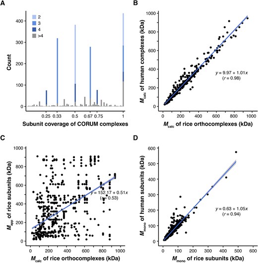
Assumed CORUM complexes do not exist in a fully assembled state in plant species. (A) Genomic-level subunit coverage of CORUM complexes to rice orthocomplexes. Coverage is defined as the ratio of the number of subunits in a rice orthocomplex to the number of subunits in its orthologous human CORUM complexes. The genome coverage of 1964 rice orthocomplexes was calculated and plotted at different subunit coverage levels. The sharp peaks are influenced by the number of members within the CORUM complexes. The various colors within each peak represent the relative proportions of different complex sizes covered. (B) Conserved predicted masses of human complexes and rice orthocomplexes. Mcalc of 436 rice orthocomplexes with 100% subunit coverage to CORUM complexes were plotted. Mapp values of the one-to-multi rice orthologs were averaged in Mcalc calculation (Fig. 1A). (C) CORUM complex subunits rarely exist in a fully assembled complex. Mapp values of subunits of the 258 rice orthocomplexes were obtained from the reference rice CFMS datasets. (D) Conserved masses of human CORUM subunits and rice orthocomplex subunits. A scatter plot shows conserved Mmono values between human and rice subunits that assemble into the known complexes. The rice orthocomplexes with 100% subunit coverage to CORUM complexes were plotted.
To assess variability in the sizes of the rice and human orthologs, we compared predicted protein complexes within the 436 human and rice orthocomplexes that shared 100% subunit coverage (Fig. 2B; Supplemental Table S2B). The Mcalc value was determined by summing the monomeric masses of individual subunits within an orthocomplex. In Fig. 2B, we illustrate that rice and human orthocomplexes exhibit similar complex sizes when considering Mcalc based on the calculated masses of the summed subunits (r = 0.986 and slope = 1.01), indicating that most complexes possess similar masses. Among these 436 orthocomplexes, 258 had detected subunit(s) in the SEC datasets. However, when Mcalc values of these highly conserved rice orthocomplexes were compared to their subunit Mapp values measured in the rice SEC experiments, a low correlation was found (Fig. 2C, r = 0.53 and R2 = 0.28). The lack of correlation in Fig. 2C indicates that the Mapp of rice orthocomplexes from SEC experiments do not align with their calculated sizes. To reinforce that the low correlation shown in Fig. 2C was not due to differences in Mmono of subunits in these 258 orthocomplexes, we found a strong positive correlation between Mmono values for this subset of human and rice orthocomplex subunits (Fig. 2D).
Furthermore, 25 proteins from the rice orthocomplexes with 100% subunit coverage had Rapp ≤ 1.6 and were therefore considered likely monomers. The existence of monomeric subunit pools and partially assembled complexes can explain the large number of data points falling well below the diagonal in Fig. 2C. Data points above the diagonal may reflect novel complexes in which CORUM orthocomplexes and/or subcomplexes interact with unknown proteins. These results are consistent with previous observations [6, 12, 17, 18] and indicate that CORUM subunits detected in CFMS experiments rarely agree with the predicted mass of the fully assembled state.
Benchmark identification
We extracted reproducible protein elution profiles from the reference rice SEC datasets [10]. There were 3426 proteins present in both of the two SEC replicates, and 197 had multiple peaks that arose when the protein existed in multiple multimerization states. We deconvolved these multiple peaks to generate 350 reproducible peaks, and a total of 2618 protein subunits with Rapp > 1 were used as the rice SEC reference profiles. We further curated rice orthocomplexes with subunit coverage greater than or equal to 2/3 in the rice SEC profiles. Among the 920 orthocomplexes meeting this coverage threshold, 531 orthocomplexes had at least one rice subunit detected by the rice SEC reference profiles, and 287 of these 531 orthocomplexes had at least two rice subunits detected. After eliminating redundant orthocomplexes, 103 rice orthocomplexes were selected for further analysis by integrating rice orthocomplexes with the rice SEC data. Clustering analysis was performed across the 103 rice orthocomplexes one by one to predict the composition of subcomplexes. The results of the clustering analysis, including essential details such as cluster composition, singleton, statistical significance, and size evaluation, are reported in Supplemental Table S3 and illustrated in Supplemental Figs. S2 and S3. More specifically, in Supplemental Fig. S2, we plotted Mapp versus Mcalc of the identified subcomplexes after the clustering analysis, demonstrating the existence of partially assembled complexes in the rice cell extract. Additionally, SEC profile plots illustrating co-elution patterns of the clustering analysis results are generated in Supplemental Fig. S3.
During the process of clustering analysis, subunits within each rice orthocomplex were clustered based on their profiles and distances. The outcome of this analysis included 162 subcomplexes/complexes from the 103 rice orthocomplexes (Fig. 3A; Supplemental Figs. S2 and S3; Supplemental Table S3). Random sampling was conducted a large number of times, specifically 134 350 times, which is equal to 50 times the total number of the rice SEC reference profiles in our dataset. Supplemental Fig. S4 displays the random empirical distributions for various subcomplex sizes. The P-values and FDR values for the 162 subcomplexes/complexes are reported in Supplemental Table S3, with 112 of them having P-values <5% and the corresponding FDR values less than 7%. After removing redundancies from the list of 112, and discarding potential monomers (Rapp ≤ 1.6), we identified 79 unique subcomplexes/complexes with small P-values (Supplemental Table S4).
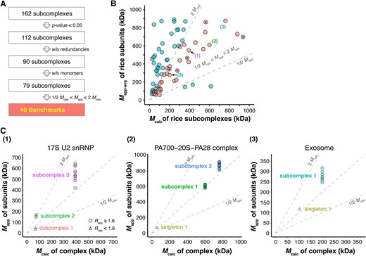
Useful benchmarks near the diagonal. (A) A process flow to identify benchmarks from the rice data. (B) Benchmark subcomplexes/complexes of rice with matched Mcalc and Mapp-avg are rendered in pink (in the middle). Asterisks (*) indicate fully assembled CORUM orthocomplexes. Numbers in parentheses point out predicted subcomplexes present in the corresponding panels in C. (C) Mcalc values of predicted subcomplexes and Mapp values of subunits of the subcomplexes. Benchmark subcomplexes (P-values = .0) are highlighted in bold text.
We proceeded to compare their Mapp and Mcalc values using the criterion defined in Formula (6) for this set of 79 subcomplexes/complexes (Fig. 3B; Supplemental Table S4). In comparison to Fig. 2C, Fig. 3B exhibits considerably fewer data points below the diagonal. This is because a subcomplex comprises fewer subunits than the CORUM orthocomplex. Therefore, the reduction in Mcalc values brought them closer to the Mapp values obtained from the SEC experiment. This result indicates that our algorithm successfully identified more reliable subcomplex formations. In Fig. 3B, those subcomplexes/complexes with elevated Mapp greater than two times Mcalc might be attributable to undetected or unknown subunits in the complexes with non-spherical shapes, or unknown subunit stoichiometries. Among the set of 79 subcomplexes/complexes, 40 demonstrated substantial agreement between Mapp and Mcalc, as shown in Fig. 3B, meeting the criterion of Formula (6).
These 40 subcomplexes or complexes were stable subcomplexes/complexes supported by both statistically significant P-values and consistent apparent masses (Fig. 3B and3C; Supplemental Table S4). They could serve as benchmarks for evaluating CFMS predictions. Additionally, within these 40 benchmarks, our algorithm identified 8 fully assembled CORUM orthocomplexes. These fully assembled complexes met the criteria of containing all CORUM subunits, being statistically significant, and having similar Mapp and Mcalc values according to Formula (6). A summary list of these 40 benchmarks is provided in Table 1, with additional details in Supplemental Table S5.
Predicted subcomplexes that could be used as benchmarks to evaluate CFMS-based protein complex predictions
| CORUM complex | Rice subcomplex IDs (# of subunits orthocomplex) | Subcomplex prediction P-value | Mcalc of subcomplex (kDa) | Mapp-avg of subcomplex (kDa) | # of CORUM subunits predicted/total # of CORUM subunits |
|---|---|---|---|---|---|
| 17S U2 snRNP | Subcomplex 3 (11) | .000008 | 392.7 | 550.0 | 9/33 |
| Gamma-BAR-AP1 complex | All proteins defined in the complex by Gaussian peak distance before clustering (3) | .004744 | 391.6 | 421.3 | 5/9 |
| APPBP1-UBA3 complex | Only 2 proteins in the complex before clustering (2) | .000947 | 108.7 | 121.3 | 2/2 |
| RNA polymerase II holoenzyme complex | Subcomplex 1 (2) | .010076 | 50.5 | 68.2 | 2/24 |
| RNA polymerase II holoenzyme complex | Subcomplex 3 (8) | .000008 | 460.2 | 636.4 | 7/24 |
| RNA polymerase II holoenzyme complex | Subcomplex 4 (3) | .011642 | 201.5 | 372.4 | 3/24 |
| C complex spliceosome | Subcomplex 2 (5) | .000252 | 880.0 | 730.4 | 5/80 |
| CAPZalpha-CAPZbeta complex | Only 2 proteins in the complex before clustering (2) | .030328 | 61.7 | 89.5 | 2/2 |
| CCT complex (chaperonin containing TCP1 complex) | All proteins defined in the complex by Gaussian peak distance before clustering (10) | .000008 | 937.1 | 698.2 | 8/8 |
| Prefoldin complex | All proteins defined in the complex by Gaussian peak distance before clustering (6) | .000008 | 99.1 | 136.8 | 6/6 |
| SEC23-SEC24 adaptor complex | All proteins defined in the complex by Gaussian peak distance before clustering (3) | .000069 | 197.6 | 341.0 | 2/2 |
| CSA-POLIIa complex | Subcomplex 1 (6) | .000008 | 301.8 | 438.7 | 6/13 |
| CUL4A-DDB1-RBBP5 complex | Subcomplex 1 (3) | .031703 | 278.6 | 325.9 | 3/3 |
| EIF2B1-EIF2B2-EIF2B3-EIF2B4-EIF2B5 complex | All proteins defined in the complex by similarity before clustering (5) | .000008 | 563.4 | 863.2 | 5/5 |
| Elongator holo complex | All proteins defined in the complex by Gaussian peak distance before clustering (3) | .000122 | 305.4 | 590.2 | 3/4 |
| ESCRT-III complex | Only 2 proteins in the complex before clustering (2) | .013789 | 98.8 | 57.9 | 4/10 |
| Exosome | Subcomplex 1 (7) | .000008 | 199.9 | 278.1 | 7/11 |
| FIB-associated protein complex | Subcomplex (ortho-paralog) 2 (4) | .000023 | 49.8 | 90.1 | 1/6 |
| HCF-1 complex | Subcomplex 1 (6) | .000008 | 177.3 | 352.0 | 2/18 |
| KAT2A-Oxoglutarate dehydrogenase complex | Subcomplex (ortho-paralog) 1 (2) | .000122 | 108.8 | 193.6 | 1/4 |
| KAT2A-Oxoglutarate dehydrogenase complex | Subcomplex 1 (3) | .002040 | 109.5 | 114.8 | 2/4 |
| LSm1–7 complex | Subcomplex 2 (4) | .000642 | 46.6 | 78.3 | 4/7 |
| LSm2–8 complex | Subcomplex 2 (5) | .000863 | 63.1 | 94.6 | 5/7 |
| MCM2-MCM4-MCM6-MCM7 complex | All proteins defined in the complex by similarity before clustering (4) | .000046 | 377.6 | 466.3 | 4/4 |
| Membrane protein complex (VCP, UFD1L, SEC61B) | Subcomplex (ortho-paralog) 2 (2) | .000405 | 538.7 | 563.7 | 1/3 |
| mRNA decay complex (UPF1, UPF2, UPF3B, DCP2, XRN1, XRN2, EXOSC2, EXOSC4, EXOSC10, PARN) | Subcomplex 1 (3) | .004362 | 173.7 | 293.0 | 3/10 |
| p400-associated complex | Subcomplex 1 (4) | .001597 | 346.2 | 614.7 | 3/6 |
| PA700-20S-PA28 complex | Subcomplex 1 (15) | .000008 | 600.7 | 610.7 | 11/36 |
| PA700-20S-PA28 complex | Subcomplex 2 (21) | .000008 | 761.6 | 876.6 | 15/36 |
| Parvulin-associated pre-rRNP complex | Subcomplex (ortho-paralog) 1 (3) | .000290 | 49.7 | 91.1 | 1/12 |
| RAF1-PPP2-PIN1 complex | Subcomplex 1 (2) | .003018 | 121.9 | 198.7 | 2/5 |
| Retromer complex (SNX1, SNX2, VPS35, VPS29, and VPS26B) | All proteins defined in the complex by similarity before clustering (3) | .002559 | 248.0 | 211.7 | 4/5 |
| Ribosome, cytoplasmic | Subcomplex 2 (2) | .001604 | 42.3 | 68.5 | 2/80 |
| SNW1 complex | Subcomplex 1 (3) | .042039 | 268.6 | 223.1 | 2/18 |
| SNW1 complex | Subcomplex 2 (4) | .002040 | 559.1 | 751.7 | 3/18 |
| SNW1 complex | Subcomplex 3 (5) | .000008 | 50.1 | 90.8 | 1/18 |
| Spliceosome | Subcomplex 1 (3) | .000733 | 64.3 | 93.8 | 4/143 |
| Spliceosome | Subcomplex 2 (2) | .010122 | 57.5 | 61.8 | 2/143 |
| TBCD-ARL2-tubulin (beta-TBCE complex) | Subcomplex 1 (2) | .000970 | 146.7 | 282.0 | 2/4 |
To further justify the machine learning approach, we applied the method to randomly shuffled rice proteins. Specifically, we randomly permuted the protein IDs among the total of 42 160 rice proteins, with 2377 of them having SEC profiles. This permutation generated a random dataset where a SEC profile (if available) did not correspond to its true protein but was instead assigned to a random protein. We conducted the entire process of benchmark analysis on the shuffled data, including CORUM ortholog mapping, SOM clustering analysis, statistical significance testing, and comparison of the Mapp and Mcalc values. Among multiple random simulations with shuffled data, we typically identified either no benchmark or one benchmark.
Confirmation of monomer identification by the algorithm
Within the set of 103 CORUM orthocomplexes, there existed a list of 50 proteins with small Rapp values (Rapp ≤ 1.6), likely being monomers or multimers with a restricted type of binding partner (Supplemental Table S6). This list, derived directly from the original input data, served as prior information to evaluate and validate the accuracy of our algorithm in discerning monomeric proteins within orthocomplexes. None of these 50 potential monomers were predicted to form subcomplexes, confirming that the algorithm effectively distinguishes monomeric proteins from those likely to be involved in larger complex assemblies.
Structural validation of RNA polymerase II subcomplexes
We identified several novel subcomplexes using our two-stage clustering approach. To validate these predictions, we focused on RNA polymerase II (Pol II) as a model example (Fig. 4). While the solved structure of rice Pol II is unavailable, we mapped the rice subunits onto the human Pol II structure (PDB: 6O9L). Using the rice CFMS data, we identified 12 reproducible subunits of the Pol II complex, including RPB3, RPB9, and RBP11a, which exhibited multiple resolvable peaks (Fig. 4A). Our clustering method assigned these subunits into four distinct subcomplexes, with subcomplexes 1, 3, and 4 showing significant P-values (≤.01), while subcomplex 2 did not (P-value = 0.56), suggesting monomeric forms for TFIIB and RPB9 (Fig. 4B). To further validate the predictions, we compared the Mapp values of the subcomplexes to their Mcalc values, supporting the presence of three significant subcomplexes (Fig. 4B and4D). We also used the AlphaFold-Multimer algorithm to explore potential interactions among subunits. The highest-confidence interaction was observed between RPB3 and RBP11, supporting the subcomplex 1 prediction (Fig. 4C). Structural mapping of the predicted subcomplexes onto the holoenzyme structure (PDB: 6O9L) showed consistency with known features, including the TFIIH and Pol II complexes (Fig. 4D). These findings support the existence of discrete RNA Pol II subcomplexes and highlight the utility of CFMS data in uncovering regulated assembly events. Our results suggest that these subcomplexes may also exist in the cytosol, reflecting potential functional roles beyond the nucleus. Importantly, our approach is not specific to plants and can be applied to other species to detect partial complex assembly.
![Validation of subcomplexes predicted in CORUM RNA polymerase II complex. (A) Protein elution profiles of subunits in each predicted subcomplex. Profiles from the second replicate are shown in Supplemental Fig. S3. (B) Mcalc values of predicted subcomplexes and Mapp values of their subunits. Circles indicate multimers, while triangles represent monomers (Rapp ≤ 1.6). (C) dimerization predictions between subcomplex subunits using AlphaFold Multimer [32]. AlphaFold-Multimer was run on COSMIC2 to predict the top five models [33]. Each value in the table represents the mean ranking confidence score (ipTM + pTM) ± standard deviation. (D) Structural validation of predicted subcomplexes. Predicted subcomplexes were searched in the RCSB protein data Bank (https://www.rcsb.org/). The structure of the fully assembled CORUM RNA polymerase II complex is available (PDB: 6O9L). (1) undetected subunits in the CFMS dataset are shown in gray. (2)–(4) subcomplexes were predicted in B. Mcalc and Mapp values of predicted rice subcomplexes are summarized next to the corresponding subcomplex structures.](https://oup.silverchair-cdn.com/oup/backfile/Content_public/Journal/bib/26/2/10.1093_bib_bbaf154/1/m_bbaf154f4.jpeg?Expires=1750198345&Signature=DxJBIyEWlbiyDwaNDCGV9rLv6jJgbuRbUppMrdGw2W48aug8t7bbRbmzycKa0TwMcufOvCe~nzzB323baGBe1BnZpARMEfZt4FtvHt5KYqHfldYfveHv4KBSuF6tpwgYL-spIEzcVWNTh4UUIn1cjPteBBVOEXxDVWjh5B3arfKT-uH5xa2lbvXIS0FnY~9bd3N9v6uFDx4~AQgpEqY7CEUWY0kYMywX8yOmhTIopuBW4ouBgVb4gNLMtiK3ovtWcReL98V1rrLhrPeBCx17MGAy-baxUjN4KY2jbZ9LTyP6hLSeZmZskT1rusw7YrSWcZ-G6UxmjHEKHhiNGzyDdA__&Key-Pair-Id=APKAIE5G5CRDK6RD3PGA)
Validation of subcomplexes predicted in CORUM RNA polymerase II complex. (A) Protein elution profiles of subunits in each predicted subcomplex. Profiles from the second replicate are shown in Supplemental Fig. S3. (B) Mcalc values of predicted subcomplexes and Mapp values of their subunits. Circles indicate multimers, while triangles represent monomers (Rapp ≤ 1.6). (C) dimerization predictions between subcomplex subunits using AlphaFold Multimer [32]. AlphaFold-Multimer was run on COSMIC2 to predict the top five models [33]. Each value in the table represents the mean ranking confidence score (ipTM + pTM) ± standard deviation. (D) Structural validation of predicted subcomplexes. Predicted subcomplexes were searched in the RCSB protein data Bank (https://www.rcsb.org/). The structure of the fully assembled CORUM RNA polymerase II complex is available (PDB: 6O9L). (1) undetected subunits in the CFMS dataset are shown in gray. (2)–(4) subcomplexes were predicted in B. Mcalc and Mapp values of predicted rice subcomplexes are summarized next to the corresponding subcomplex structures.
Benchmark identification in Arabidopsis
We applied the same pipeline to Arabidopsis, as outlined in Fig. 1. InParanoid was used to identify orthologs between 20 834 human proteins and 35 368 Arabidopsis proteins, resulting in 3227 OGs (Supplemental Table S1B). Of the 3047 human complexes in CORUM, 1985 (65.1%) had at least one orthologous subunit in Arabidopsis. Among these, 970 complexes had >2/3 subunit coverage (Supplemental Table S7). Using a previously published Arabidopsis SEC dataset [27], we applied the same filtering criteria as for the rice data to identify reproducible protein elution profiles. This yielded 1738 subunits with Rapp > 1. Of the 970 orthocomplexes, 289 had at least one detected Arabidopsis subunit, and 184 had at least two. After removing redundant complexes, 63 orthocomplexes were selected for further analysis (Supplemental Table S8). Similar to rice, there was poor agreement between Mapp of Arabidopsis subunits and Mcalc of the assumed fully assembled Arabidopsis orthocomplexes (Supplemental Fig. S5).
We used the same two-stage clustering algorithm applied to rice, identifying 23 Arabidopsis benchmarks with statistically significant P-values and matching Mapp and Mcalc values (Fig. 5A; Supplemental Figs. S6 and S7; Supplemental Table S9). To analyze the extent to which subcomplexes were conserved in a monocot and dicot species, we compared the 40 rice subcomplexes and 23 Arabidopsis subcomplexes. A stringent comparison, requiring the complete overlap of all subunits between an Arabidopsis subcomplex and its corresponding rice subcomplex, was limited to only 5 predicted benchmarks. This was largely due to non-overlapping proteome coverages obtained from different tissue types and different mass spectrometers. As an alternative approach, we compared Mapp values of subcomplexes predicted in both species for cases in which at least one conserved subunit was detected (Fig. 5B; Supplemental Table S10). Eleven subcomplexes were represented in the datasets from both species and showed the same or similar Mapp values, suggesting conserved assemblies. This result showcases the generalizability of our benchmark identification in species that diverged >100 million years ago. However, the agreement was not absolute, as three rice orthologs had an elevated Mapp compared to their Arabidopsis counterparts (Fig. 5B).
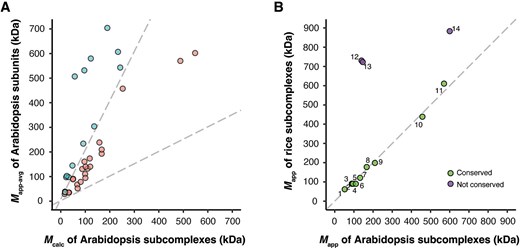
Benchmarks identified in Arabidopsis. (A) Benchmark subcomplexes/complexes of Arabidopsis with matched Mcalc and Mapp-avg are rendered in pink (in the middle). (B) Conservation of rice and Arabidopsis subcomplexes. Mapp values of rice benchmarks and Mapp values of their orthologous Arabidopsis benchmarks were plotted. The conserved benchmarks (on the diagonal line) and non-conserved ones (above the diagonal line) are reported in Supplemental Table S10.
Discussion
Protein correlation profiling (also known as CFMS) is a powerful tool to predict the multimerization state, composition, and localization of endogenous protein complexes. As mass spectrometry coverage and subcellular fractionation methods improve, CFMS will increasingly link in vitro biochemistry with cell function. A key limitation in CFMS is the lack of data on true protein multimerization states. Solved CORUM structures certainly exist in cells, but the extent to which the fully assembled state dominates the subunit pools is not known. Our analyzes of Arabidopsis and rice soluble extracts indicate that CORUM orthocomplexes are rarely fully assembled. We anticipate the same to be true in non-plant systems. This study introduces robust experimental methods and statistical/machine learning approaches to identify more reliable benchmarks that better reflect the multimerization states of CORUM orthologs in cell extracts. Tools like InParanoid and EggNOG enable accurate mapping of orthologs across species, and the two-stage clustering algorithm developed here successfully predicts reliable complexes. Evolutionarily conserved multimeric assemblies were identified, but benchmarks cannot be transferred across species or kingdoms without testing for multimerization variability.
Accurate benchmark databases will improve CFMS predictions, though some errors, such as chance co-elution, remain a challenge due to high sample complexity. Optimizing cluster numbers with benchmarks or conducting series IEX and SEC separations may help, but increased sample fractionation will be key. Future advances in mass spectrometry and computational tools will enhance our ability to analyze protein multimerization dynamics.
CORUM complexes are not reliable benchmarks for protein complex predictions.
Ortholog mapping identifies evolutionarily conserved CORUM complexes.
Integrating evolutionary conservation from CORUM and co-elution patterns from CFMS enhances benchmark protein complexes.
Conflict of interest: None declared.
Funding
This work was supported by the National Science Foundation (NSF) Plant Genome Research Project 1951819 to D.B.S.
Data availability
The source code and sample input data for the clustering analysis are publicly available on GitHub (https://github.com/yangpengchengstat/R-code-S4_Class-protein-clustering-based-on-data-integration-of-corum-and-inparanoid.git). The package at the GitHub link contains comprehensive information on running the code, description of the input data, and steps of performing hyperparameter tuning.
References
Author notes
Pengcheng Yang and Youngwoo Lee contributed equally to this work.
