


Abstract
Identifying spatial domains is critical for understanding breast cancer tissue heterogeneity and providing insights into tumor progression. However, dropout events introduces computational challenges and the lack of transparency in methods such as graph neural networks limits their interpretability. This study aimed to decipher disease progression-related spatial domains in breast cancer spatial transcriptomics by developing the three graph regularized non-negative matrix factorization (TGR-NMF). A unitization strategy was proposed to mitigate the impact of dropout events on the computational process, enabling utilization of the complete gene expression count data. By integrating one gene expression neighbor topology and two spatial position neighbor topologies, TGR-NMF was developed for constructing an interpretable low-dimensional representation of spatial transcriptomic data. The progressive lesion area that can reveal the progression of breast cancer was uncovered through heterogeneity analysis. Moreover, several related pathogenic genes and signal pathways on this area were identified by using gene enrichment and cell communication analysis.
Introduction
Breast cancer is the most common malignant tumor among women, accounting for about a quarter of the global new cancer cases [1]. High incidence rate and significant heterogeneity make breast cancer the focus of global research and clinical attention [2]. The heterogeneity of breast cancer is reflected in the significant differences in disease manifestation, progress speed and treatment response of patients, which makes the diagnosis, treatment, and prognosis of breast cancer complicated [3]. Although recent studies have improved our understanding of breast cancer, there are still many challenges to fully reveal its heterogeneity.
In recent years, spatially resolved transcriptomic technology has provided gene expression profile information while preserving the spatial position information of cells [4], which is crucial for revealing how gene expression in cells is influenced by the surrounding microenvironment [5]. The existing spatially resolved transcriptomic techniques can be roughly divided into two categories: the first category is in-situ hybridization or in-situ sequencing technologies, such as seqFISH [6], seqFISH+ [7], MERFISH [8], osmFISH [9], STARmap [10], and FISSEQ [11]. These technologies can analyze hundreds of genes at subcellular resolution within a single cell, but there are limitations in detecting a large number of genes [12]. The second type is next-generation sequencing-based technologies, such as ST [13], SLIDE-seq [14], SLIDE-seqV2 [15], HDST [16], and 10x Visium [17]. These technologies can detect thousands of genes, but their spatial resolution is low (10-100|$\mu{m}$|), and each metric position is called a spot [5]. These different spatially resolved transcriptomic techniques enable us to more accurately characterize tissue heterogeneity and cellular function.
It cannot be denied that these sequencing techniques may face sensitivity limitations when detecting low abundance genes, which can result in the expression levels of some genes being incorrectly measured as 0 (dropout events) [18]. There are two strategies to address this issue: deletion and interpolation [19]. The deletion strategy usually retains genes with sufficient expression levels in most spots. For example, Avesani et al. deleted genes expressed in fewer than 10 spots to reduce noise. The interpolation strategy compensated for the impact of dropout events by estimating the lost data [20]. For example, Liu et al. proposed a dual factor smoothing method that interpolated the gene expression profile of the spatial transcriptome by simultaneously considering gene expression information and spatial position information in Euclidean space [21]. Although these methods can alleviate the impact of dropout events to some extent, they can also lead to the loss of useful information or the introduction of additional uncertainty. Thus, how to effectively handle dropout events in high-dimensional and sparse gene expression data remains an important challenge.
In spatially resolved transcriptomic research, detecting spatial domains with consistent gene expression is a key analytical task [22]. These spatial domains are composed of multiple cells and are typically associated with the anatomical structure and specific functions of the tissue [23]. Clustering algorithms are widely used to identify these spatial domains. Early methods (K-means and Louvain algorithm [24]) only considered high-dimensional and sparse gene expression information while ignoring spatial dependency, which may result in discontinuous clustering results [25]. To improve the identification performance of spatial domains, researchers developed two methods in the early stages that incorporated spatial position information into clustering [26]. The first method assumed that cells that were physically far apart were not very similar to each other, but, in practice, cells of the same type could often be far apart [27]. The second method used the Markov random field framework to annotate cell types by combining the gene expression characteristics of each cell with the clustering membership of its physical neighbors [26]. Although these methods attempt to simulate the microenvironment composition of cells, it is difficult to scale to large spatial datasets and requires prior knowledge of the number of clusters.
Based on these early explorations, many probabilistic learning methods and deep learning methods have been developed to identify spatial domains by utilizing spatial position information. For example, Zhao et al. proposed the BayesSpace model based on the fully Bayesian statistical method, which cleverly incorporated spatial prior knowledge to facilitate the division of adjacent positions into the same cluster [28]. Dries et al. developed a Giotto model based on Hidden Markov random field for detecting spatial domains by utilizing the dependency relationships between spots [29]. Although these methods can cluster spots or cells into different groups, the lack of flexibility with different modalities has made them less versatile. Hu et al. proposed a SpaGCN model by constructing an undirected weighted graph to capture the spatial dependence of data [5]. Xu et al. constructed an SEDR model by combining gene expression representations from deep autoencoder networks with spatial information embedded in variational graph autoencoder modules [2]. Dong et al. developed a STAGATE model by using graph attention autoencoders to aggregate spatial and gene expression information [30]. Although these deep learning methods can efficiently cluster spots into different domains, they may face challenges such as relatively high computational complexity or limited interpretability.
Inspired by the ability of non-negative matrix factorization (NMF) to decompose high-dimensional data into interpretable feature combinations [31–33], this study introduced a novel threegraph regularized non-negative matrix factorization (TGR-NMF) model to decipher progressive lesion areas in breast cancer. By utilizing gene expression counts and positional coordinate data, TGR-NMF generated robust and meaningful low dimensional representations that are more suitable for identifying spatial domain tasks. The experimental results of spatial domain identification in breast cancer spatial transcriptomics showed that TGR-NMF was superior to the existing seven classical methods.
Materials and methods
Data description
In this study, we utilized two spatially resolved transcriptomic datasets of human breast cancer (HBRC) generated by 10x Genomics Visium. The first HBRC dataset, comprising 3798 spots and 36 601 genes, was downloaded from https://www.10xgenomics.com/resources/datasets/human-breast-cancer-block-a-section-1-1-standard-1-1-0. Xu et al. manually divided the histological images into 20 domains based on H&E staining and pathological features (Fig. 3(a)) [2]. Within these domains, four main morphological types were represented: ductal carcinoma in situ/lobular carcinoma in situ (DCIS/LCIS), invasive ductal carcinoma (IDC), tumor surrounding regions with low features of malignancy (Tumor edge), and healthy tissue (Healthy) (Fig. 5(a)). Similar to the approaches in [4] and [34], the spot types annotated by Xu et al. were regarded as the gold standard for evaluating the performance of spatial domain identification in breast cancer. The second HBRC dataset, consisting of 4784 spots and 28 402 genes, was obtained from https://zenodo.org/records/4739739. This dataset includes six main morphological types—artefact, invasive cancer with stroma and lymphocytes, lymphocytes, necrosis, stroma, and TLS—annotated by Wu et al. [35]. To describe the two datasets mentioned above, we adopt the following mathematical notation: Let |$m$| and |$n$| denote the total number of genes and the total number of spots, respectively. We define |$\overline{X}=[\overline{X}_{1}, \ldots , \overline{X}_{i}, \ldots , \overline{X}_{n}] \in \mathbb{R}^{m \times n}$| as the original gene expression count matrix, where |$\overline{X}_{i}=(\overline{X}_{1i}, \ldots , \overline{X}_{mi})^{T}$| represents the |$i$|th column of the matrix |$\overline{X}$| corresponding to the |$i$|th spot feature vector. Additionally, we denote the original position coordinate matrix as |$\overline{P}=[\overline{P}_{1}, \ldots , \overline{P}_{i}, \ldots , \overline{P}_{n}] \in \mathbb{R}^{2 \times n}$|, where |$\overline{P}_{i}=(\overline{P}_{1i}, \overline{P}_{2i})^{T}$| is the |$i$|th column of the matrix |$\overline{P}$|, representing the |$i$|th spot position vector.
Overview of deciphering disease progression-related spatial domains in breast cancer spatial transcriptomics
TGR-NMF is an interpretable model for identifying interesting spatial domains that reveal breast cancer progression by using spatial transcriptomic data. TGR-NMF accounts for the impact of dropout events in computation and introduces three graph regularization terms by integrating gene expression count data and positional coordinate information. The workflow for deciphering spatial domains in breast cancer spatial transcriptomics was shown in Fig. 1. Firstly, the unitization strategy was adopted to process the gene expression count matrix and position coordinate matrix. Secondly, TGR-NMF was constructed by integrating three distinct graph regularization terms to obtain a low-dimensional representation of the gene expression count data. The construction of these regularization terms involves heat kernel weighting for the gene expression count matrix, cosine similarity and heat kernel weighting for the position matrix. Next, the K-means algorithm was employed to identify the spatial domains based on the obtained low-dimensional representation. To validate the ability of the low-dimensional representation in identifying spatial domains, uniform manifold approximation and projection (UMAP) analysis and partition-based graph abstraction (PAGA) trajectory inference analysis were performed. Furthermore, heterogeneity analysis was performed by setting different numbers of clusters to uncover disease progression-related spatial domains (see section heterogeneity analysis of breast cancer tissue). Finally, differential expression analysis (DEA), Kyoto Encyclopedia of Genes and Genomes (KEGG) pathway enrichment analysis, Gene Ontology (GO) enrichment analysis, and cell communication analysis were performed to identify key genes and signal pathways related to breast cancer.
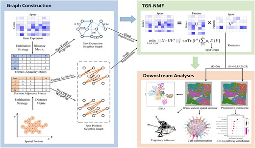
The workflow for deciphering spatial domains in breast cancer spatial transcriptomics.
Unitization strategy and distance measure
Dropout events (false zero counts) in spatial transcriptomic data can lead to inaccuracy in vector-based numerical calculations, thereby affecting the identification of spatial domains in breast cancer. Generally, there are two strategies for handling dropout events: one is to delete genes that are expressed as zero in the majority of spots, and the other is to interpolate genes that are expressed as zero in only a few spots. The former may result in the loss of valuable information (non-zero counts), and the latter would also lead to the inaccuracies in vector-based numerical calculations due to the introduction of new uncertainties.
Based on the following two motivations: (1) fully utilize all valid information of the gene expression count matrix. (2) Reduce the impact of dropout events on computation. We proposed the following strategy for unitizing spot feature vector |$\overline{X}_{i}$|
where |$||\cdot ||$| represents the 2-norm of the vector. Under the unitization strategy (1), the Euclidean distance between the unitized spot feature vectors |$X_{p}$| and |$X_{q}$| can be simplified to
where |$X_{p}^{T}$| represents the transpose of |$p$|th unitized spot feature vector, |$X_{gp}$| and |$X_{gq}$| represent the unitized count of the |$g$|th gene in the |$p$|th and |$q$|th spot feature vector, respectively.
According to (2), dropout events introduce uncertainty in computation by the product of zero elements and their corresponding non-zero (positive) elements. It is observed that the uncertainty increases with the magnitude of positive elements multiplied by zero elements. Therefore, uniting the spot feature vectors effectively reduces the contribution of large counts, thereby minimizing the uncertainty associated with their multiplication with zero elements. It should be noted that the Euclidean distance (2) between unitized spot feature vectors is independent of the length of the vectors and depends solely on the angle between the two vectors. For metric purposes, we let |$||\overline{X}_{p}-\overline{X}_{q}||_{\overline{X}UE}=||X_{p}-X_{q}||$| denote the |$\overline{X}UE$|-distance between original spot feature vectors |$\overline{X}_{p}$| and |$\overline{X}_{q}$| from the gene expression count data (matrix) |$\overline{X}$|. It should be noted that one |$\overline{X}_{q}$| corresponds to a unique unitized spot feature vector |$X_{q}$|, while one |$X_{q}$| may correspond to all other original spots besides |$\overline{X}_{q}$|. Similarly, the |$K$| neighbors of |$X_{q}$| correspond to more spots in the original spot space.
The schematic diagram of |$\overline{X}UE$|-distance between spot feature vectors and their 2-nearest neighbors in the case of two-dimensional (two-gene) data was shown in Fig. 2. Due to the non-negativity of gene expression counts, the original spot feature vectors are distributed only in the first quadrant and are transformed into points on the arc DE after unitization by (1). For example, all spots on the ray OA are transformed into |$S_{2}$| after unitization. The |$\overline{X}UE$|-distance between any spot on ray OA and any spot on ray OB (or OC) is equal to |$l$|. As shown in Fig. 2, the original spot feature vector |$S_{1}$| has |$S_{3}$| and |$S_{4}$| as its 2-nearest neighbors under the Euclidean distance. However, under the |$\overline{X}UE$|-distance, its 2-nearest neighbors are all the spots on the three rays OA, OB, and OC, i.e. the 2-nearest neighbors of the unitized spot feature vector |$S_{2}$|.
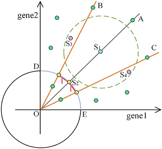
The schematic diagram of |$\overline{X}UE$|-distance between spot feature vectors and their 2-nearest neighbors in the case of two-dimensional (two-gene) data.
Due to the presence of coordinate scale differences, the length of the spot position vectors cannot effectively measure the topological relationships between spots. An alternative metric is the angle between vectors. Inspired by this, we unitized the spot position vectors |$\overline{P}_{i}$| by using a method similar to (1)
Based on the unitization strategy (3) mentioned above, we let
denote the |$\overline{P}UE$|-distance between original spot feature vectors |$\overline{P}_{p}$| and |$\overline{P}_{q}$| from the position coordinate data (matrix) |$\overline{P}$|, where |$cos(P_{p},P_{q})$| represents the cosine value of the angle between spot position vectors |$P_{p}$| and |$P_{q}$|.
Three graph regularized non-negative matrix factorization
Let |$\mathcal{N}_{K_{1}}(X_{q})$| denote the set of |$K_{1}$|-nearest neighbors for unitized spot feature vector |$X_{q}$| under the |$\overline{X}UE$|-distance defined in (1) and (2). Let |$L^{g-hot}=[L^{g-hot}_{pq}]_{n\times n}$| denote the Laplacian matrix that describes the topological relationships of gene expression neighbors for the spots, where
Let |$\mathcal{N}_{K_{2}}(P_{q})$| denote the set of |$K_{2}$|-nearest neighbors for unitized spot position vector |$P_{q}$| under the |$\overline{P}UE$|-distance defined in (3) and (4). Let |$L^{p-cos}=[L^{p-cos}_{pq}]_{n\times n}$| and |$L^{p-hot}=[L^{p-hot}_{pq}]_{n\times n}$| denote Laplacian matrices which describe the topological relationships of spatial position neighbors for the spots, where
Let |$X = [X_{1},..., X_{i},..., X_{n}]$| be the unitized gene expression count matrix obtained from (1), |$||\cdot ||_{F}$| denote the Frobenius norm of the matrix, and |$\mathrm{Tr}(\cdot )$| denote the trace of the matrix. To obtain the low-dimensional representation of spatial transcriptomic data, we proposed the following TGR-NMF model:
where the regularization parameter |$\alpha $| and the weight parameters |$\mu _{1}$|, |$\mu _{2}$|, and |$\mu _{3}$| are positive constants, |$U\in \mathbb{R}^{m \times k}$| and |$V\in \mathbb{R}^{n \times k}$| represent the base matrix and the coefficient matrix, respectively. The purpose of introducing three weight parameters is to balance the contributions of the topological relationships between gene expression neighbors and the two topological relationships between spatial position neighbors. The parameters set in the experiments were presented in the discussion section. Note that |$V$| is a low-dimensional representation of spatial transcriptomic data. Hence, we identified the spatial domains of breast cancer by performing a K-means clustering algorithm on the rows of |$V$|.
Solving algorithm
Similar to references [31, 36, 37], we adopted the alternating update algorithm to solve the optimization problem (11). First, we constructed the following Lagrange function of (11)
where the non-negative matrices |$\Psi $| and |$\Phi $| are the Lagrange multiplier matrices related to the constraints |$U\geq 0$| and |$V\geq 0$|, respectively. By setting the partial derivative of Lagrange function |$\mathcal{L}$| in (12) with respect to |$U$| and |$V$| to zero, we have
By right-multiplying both sides of matrix equations (13) and (14) by |$U^{T}$| and |$V^{T}$|, respectively, we have
Without causing any confusion, we use the subscript |$ij$| in the proof below to denote the element corresponding to the |$i$|th row and |$j$|th column of the matrix. Using the KKT conditions, i.e. |$\Psi _{ij}U_{ij}=0$| and |$\Phi _{ij}V_{ij}=0$|, we have the following equations for |$U_{ij}$| and |$V_{ij}$|
From (15) and (16), the update rules for the base matrix |$U$| and the coefficient matrix |$V$| are easily obtained as follows:
Similar to references [36, 37], it is proven that the algorithm for solving TGR-NMF is convergent. The pseudocode for solving TGR-NMF was presented in Algorithm 1.

Comparison method and evaluation criteria
To evaluate the performance of TGR-NMF in breast cancer spatial domain identification, we compared it with seven existing classical methods: Seurat [24], Mclust [38], BayesSpace [28], Giotto [29], SpaGCN [5], SEDR [2], and STAGATE [30]. The last five methods are based on spatial clustering, while the first two methods are not. The characteristics of the seven competitive methods were summarized in Table 1. For a fair comparison, we conducted benchmark tests using the parameters optimized for each method [2, 5, 24, 28–30, 38]. In addition, to assess the effectiveness of the preprocessing strategy for dropout events and the three graph regularization terms incorporated into the model, we performed ablation analysis using standardized procedures.
The characteristics of seven competing spatial domain identification methods
| Methods | Model | Code | |
|---|---|---|---|
| non-spatial | Seurat [24] | Principal component analysis | R |
| Mclust [38] | Gaussian Mixture Model | R | |
| spatial | BayesSpace [28] | Bayesian model with a Markov random field | R |
| Giotto [29] | Hidden Markov random field | R | |
| SpaGCN [5] | Graph convolutional network | Python | |
| SEDR [2] | Variational graph autoencoder+masked self-supervised | Python | |
| STAGATE[30] | Graph attention autoencoder | Python |
Similar to references [2, 4, 34], Adjusted Rand Index (ARI) was used to evaluate the performance of breast cancer spatial domain identification. ARI measures the similarity between the predicted cluster labels and the ground truth labels from the gold standard by [2]. A higher ARI value indicates a greater similarity between the two sets of labels, with values ranging from -1 to 1. Let |$G=\{G_{1},G_{2},...,G_{d}\}$| and |$H=\{H_{1},H_{2},...,H_{d}\}$| denote the sets of the ground truth labels and the predicted cluster labels, respectively. The ARI is defined as follows:
where |$d$| is the number of spatial domains, |$ {a}\choose{b}$| represents the number of all possible combinations of |$b$| elements chosen from the set of |$a$| elements, |$N$| is the total number of spots, |$N_{l.}$| is the number of spots belonging to |$H_{r}$| in the clustering result, |$N_{.r}$| is the number of spots belonging to |$G_{l}$| in the ground truth labels, and |$N_{lr}$| is the number of spots that belong to both the |$l$|th class in the clustering results and the |$r$|th class in the ground truth.
In addition, we also evaluated the performance of TGR-NMF in identifying spatial domains by Gold Standard Comparison Accuracy (GSCA). GSCA is defined as the percentage of spots predicted to be in the correct cluster label (compared to the ground truth label from the gold standard by Xu et al.) relative to the total number of spots and is calculated as follows:
where |$y_{i}$| and |$y_{i}^{*}$| respectively represent the ground truth label and the predicted label of the |$i$|th spot, |$N$| is the total number of spots, |$map(\cdot )$| denotes the optimal permutation function that maps predicted labels to ground truth labels and is determined using the Hungarian algorithm, |$\mathrm{I}(\cdot ,\cdot )$| denotes the indicator function, which is used to compare two values and return a binary result. Specifically, for two inputs |$d$| and |$f$|, the indicator function |$\mathrm{I}(d,f)$| is defined as
Downstream analyses
To verify the distinguishability of the identified spatial domains and uncover the gradient transition from normal tissue to cancerous tissue, we conducted UMAP analysis and PAGA trajectory inference analysis [30, 34]. Additionally, to elucidate the heterogeneity of breast cancer tissue, we performed four comprehensive biological analyses: DEA, KEGG pathway enrichment analysis [2], GO enrichment analysis [4], and cell communication analysis [4]. DEA was employed to identify key genes in the progressive lesion area (see section heterogeneity analysis of breast cancer tissue). GO and KEGG pathway enrichment analyses were conducted to elucidate the roles of differentially expressed genes (DEGs) in tumor development and to identify associated signal pathways. Cell communication analysis was performed to reveal the complex network of information transmission and interactions between cells.
Based on the low-dimensional representation generated by TGR-NMF, UMAP analysis and PAGA trajectory inference analysis were performed by using the Scanpy library in Python. DEA was conducted with the edgeR package in R, applying the parameters |$|log2FoldChange|\geq 0.8$| and |$FDR<0.05$|. KEGG pathway enrichment analysis and GO enrichment analysis were carried out using an online tool (https://www.bioinformatics.com.cn/basic_local_go_pathway_en richment_analysis_122). Cell communication analysis was performed using the CellChat package in R.
Results
Performance comparison of spatial domain identification in breast cancer spatial transcriptomics
The ARI and GSCA of TGR-NMF and seven other existing classical spatial domain identification methods (Seurat, Mclust, BayesSpace, Giotto, SpaGCN, SEDR, and STAGATE) on the first HBRC dataset were listed in Table 2. The experimental results indicated that TGR-NMF achieved the highest ARI (0.5286) in breast cancer spatial domain identification, which was 0.0674, 0.0476, 0.0036, 0.238, 0.1056, 0.1618, and 0.0342 higher than Seurat, Mclust, BayesSpace, Giotto, SpaGCN, SEDR, and STAGATE methods, respectively. Similarly, the GSCA of TGR-NMF was 0.5711, which exceeded other methods by 0.0482, 0.0635, 0.0361, 0.178, 0.1232, 0.0877, and 0.0511, respectively. Visualizations of the spatial domains identified by these eight methods were shown in Fig. 3(b)–3(i). It can be observed that the spatial domains identified by TGR-NMF were more consistent with the manually annotated domains provided by [2], and many key domains such as IDC|$\_$|2, IDC|$\_$|4, DCIS|${/}$|LCIS|$\_$|1, etc., can be correctly identified, while other methods for identifying spatial domains could not. In addition, some clusters identified by the TGR-NMF model can be annotated, with cluster 1 annotated as Healthy_1, cluster 3 annotated as Tumor_edge_2, cluster 5 annotated as DCIS/LICIS_1, cluster 7 annotated as IDC4, etc. It should be noted that not all clusters can be annotated since the obtained clustering results cannot completely overlap with the gold standard.
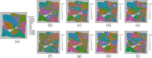
Visualization of spatial domain on the first HBRC dataset. (a) Visualization of 20 spatial domains manually annotated based on H&E staining and pathological features. (b) Visualization of spatial domain identified by TGR-NMF. (c–d) Visualization of spatial domains identified based on non-spatial clustering algorithms Seurat and Mclust. (e–i) Visualization of spatial domains identified based on spatial clustering algorithms BayesSpace, Giotto, SpaGCN, SEDR, and STAGATE.
The ARI and GSCA of eight spatial domain identification methods on the first HBRC dataset
| ARI | GSCA | |
|---|---|---|
| TGR-NMF | 0.5286 | 0.5711 |
| Seurat | 0.4612 | 0.5229 |
| Mclust | 0.4810 | 0.5076 |
| BayesSpace | 0.5250 | 0.5350 |
| Giotto | 0.2906 | 0.3931 |
| SpaGCN | 0.4230 | 0.4479 |
| SEDR | 0.3668 | 0.4834 |
| STAGATE | 0.4944 | 0.5200 |
| ARI | GSCA | |
|---|---|---|
| TGR-NMF | 0.5286 | 0.5711 |
| Seurat | 0.4612 | 0.5229 |
| Mclust | 0.4810 | 0.5076 |
| BayesSpace | 0.5250 | 0.5350 |
| Giotto | 0.2906 | 0.3931 |
| SpaGCN | 0.4230 | 0.4479 |
| SEDR | 0.3668 | 0.4834 |
| STAGATE | 0.4944 | 0.5200 |
To evaluate the generalization performance of TGR-NMF, we also conducted spatial domain identification experiments on the second HBRC dataset. Table 3 listed the ARI and GSCA of eight spatial domain identification methods. It was observed that TGR-NMF achieved the highest GSCA (0.6024), which was 0.2824, 0.2648, 0.3047, 0.3206, 0.2809, 0.1453, and 0.3164 higher than the other seven competitive methods, respectively. It should be pointed out that all methods achieved low ARI on this dataset, which is attributed to the extremely imbalanced categories of the dataset. The visualization results of eight spatial domain identification methods on the second HBRC dataset were shown in the Supplementary Fig. S1(b–i). Furthermore, in terms of Stromal type identification, the proposed method yielded results that were more consistent with the gold standard compared to the other methods.
The ARI and GSCA of eight spatial domain identification methods on the second HBRC dataset
| ARI | GSCA | |
|---|---|---|
| TGR-NMF | 0.0176 | 0.6024 |
| Seurat | 0.0076 | 0.3200 |
| Mclust | 0.0146 | 0.3376 |
| BayesSpace | 0.0052 | 0.2977 |
| Giotto | -0.0012 | 0.2818 |
| SpaGCN | 0.0041 | 0.3215 |
| SEDR | 0.0072 | 0.4571 |
| STAGATE | 0.0129 | 0.2860 |
| ARI | GSCA | |
|---|---|---|
| TGR-NMF | 0.0176 | 0.6024 |
| Seurat | 0.0076 | 0.3200 |
| Mclust | 0.0146 | 0.3376 |
| BayesSpace | 0.0052 | 0.2977 |
| Giotto | -0.0012 | 0.2818 |
| SpaGCN | 0.0041 | 0.3215 |
| SEDR | 0.0072 | 0.4571 |
| STAGATE | 0.0129 | 0.2860 |
The low-dimensional representation of spatial transcriptomic data generated by TGR-NMF plays a crucial role in both spatial domain identification and downstream analyses. Here, UMAP was employed to project the low-dimensional representation onto a two-dimensional space, facilitating the visualization of distinct spatial domains within this reduced space. The UMAP visualizations for TGR-NMF, Mclust, BayesSpace, and STAGATE were shown in Fig. 4(a)–4(d). The experimental results indicated that most spots were well-organized within their respective spatial domains, and the low-dimensional representation generated by TGR-NMF effectively separated invasive ductal carcinoma domain (tumor core region) from other domains during the clustering process. Specifically, clusters 7 and 20 (invasive ductal carcinoma domains) exhibited significant separation from other clusters, which has not been observed with other classical spatial domain identification methods. Additionally, the PAGA visualizations for TGR-NMF, Mclust, BayesSpace, and STAGATE were shown in Fig. 4(e)-4(h). It was worth noting that Fig. 4(e) clearly showed that cluster 2 within the healthy region not only maintained a close interaction relationship with cluster 1 in the same healthy region but also significantly established close communication with multiple clusters (clusters 3, 17, and 4) in the tumor edge region. This observation revealed a transition from the healthy region to the tumor edge. Additionally, the communication activity of cluster 3 in the tumor edge extended to clusters 16 and 6 in the invasive ductal carcinoma region, forming a pathway of information transmission from the tumor edge to the tumor core. This series of complex communication processes provided direct evidence for the transition from healthy regions to cancer core regions.
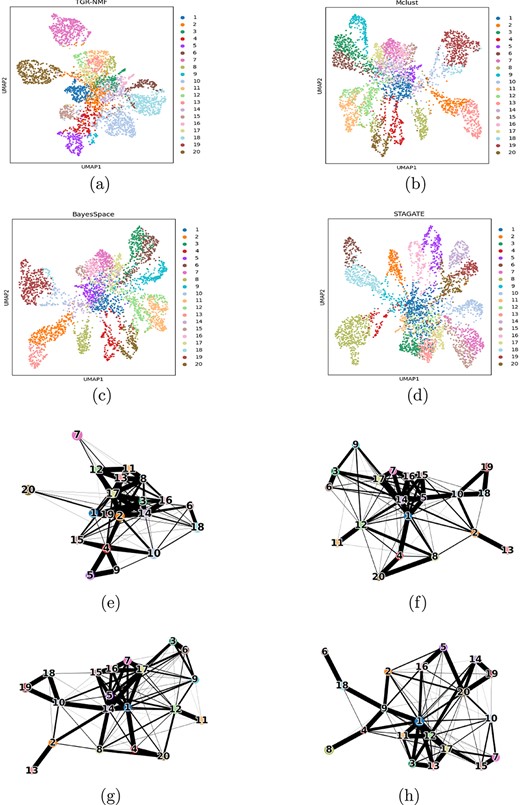
UMAP visualizations and PAGA graphs. (a–d) UMAP visualizations generated by low-dimensional representations of TGR-NMF, Mclust, BayesSpace, and STAGAE on the first HBRC dataset. (e–h) PAGA graphs generated by low-dimensional representations of TGR-NMF, McLust, BayesSpace, and STAGAE on the first HBRC dataset.
Ablation analysis of TGR-NMF
To evaluate the influence of the three graph regularization terms on the performance of TGR-NMF, ablation analysis was performed on the first HBRC dataset. Let ①, ②, and ③ denote the three graph regularization terms constructed according to (5), (7), and (8), respectively. The ARI and GSCA of the model after ablating each regularization term were detailed in Table 4. The experimental results showed that the model constructed by combining one gene expression neighbor topology and two spatial position neighbor topologies achieved the highest ARI (0.5286) and GSCA (0.5711), indicating that combining three graph regularization terms can generate a more informative low-dimensional representation. Specifically, the ARI of the proposed model increased by 0.3273, 0.1206, 0.3533, 0.0089, 0.0381, and 0.3295 compared with the models constructed after ablating each regularization term. It was worth noting that the performance of the model constructed by combining regularization terms ② and ③ was poor. Although this configuration considered the spatial location neighbor relationship between spots, it ignored the gene expression information, which is very important for spatial domain identification. Additionally, ablation analysis was also performed to validate the effect of the proposed unitization strategy on model performance. Let |$X$| and |$P$| (|$\overline{X}$| and |$\overline{P}$|) denote the (not) unified gene expression count matrix and position coordinate matrix, respectively. The ARI and GSCA of models constructed using different unitization strategies were listed in Table 5. The experimental results showed that the model’s performance significantly decreased when either both matrices were not unitized or only one matrix was unitized. The results from the ablation analysis validated the necessity and effectiveness of the TGR-NMF framework.
The ARI and GSCA of the model after ablating each regularization term on the first HBRC dataset
| ARI | GSCA | |
|---|---|---|
| ① | 0.2013 | 0.2875 |
| ② | 0.4080 | 0.4879 |
| ③ | 0.1753 | 0.2894 |
| ①+② | 0.5197 | 0.5664 |
| ①+③ | 0.4905 | 0.5413 |
| ②+③ | 0.1991 | 0.3041 |
| ①+②+③ | 0.5286 | 0.5711 |
| ARI | GSCA | |
|---|---|---|
| ① | 0.2013 | 0.2875 |
| ② | 0.4080 | 0.4879 |
| ③ | 0.1753 | 0.2894 |
| ①+② | 0.5197 | 0.5664 |
| ①+③ | 0.4905 | 0.5413 |
| ②+③ | 0.1991 | 0.3041 |
| ①+②+③ | 0.5286 | 0.5711 |
The ARI and GSCA of models constructed using different unitization strategies on the first HBRC dataset
| |$\overline{X}+\overline{P}$| | |$X+\overline{P}$| | |$\overline{X}+P$| | |$X+P$| | |
|---|---|---|---|---|
| ARI | 0.2442 | 0.4975 | 0.1581 | 0.5286 |
| GSCA | 0.3418 | 0.5453 | 0.2582 | 0.5711 |
| |$\overline{X}+\overline{P}$| | |$X+\overline{P}$| | |$\overline{X}+P$| | |$X+P$| | |
|---|---|---|---|---|
| ARI | 0.2442 | 0.4975 | 0.1581 | 0.5286 |
| GSCA | 0.3418 | 0.5453 | 0.2582 | 0.5711 |
Heterogeneity analysis of breast cancer tissue
To uncover the high heterogeneity of breast cancer tissue, spots were divided into spatial domains with different thickness by setting different cluster numbers (K=10, 15, 20, 25), as shown in Fig. 5(b)–5(e). As expected, highly heterogeneous tumor regions showed more detailed partitioning when increasing the number of clusters, while healthy regions with lower heterogeneity remained largely consistent at different clustering resolutions, indicating that TGR-NMF has good robustness. When the number of clusters was set to 20, higher resolution allows us to observe heterogeneity within the tumor in more detail, such as domains 13 and 15 (Fig. 5(d)). It was worth noting that regardless of the number of clusters set, the healthy region in the upper right corner was always divided into cluster 1 located at the center and with a relatively constant size (occupying a larger area), as well as other clusters that gradually subdivided as the number of clusters increased (occupying a smaller area). Based on the above observations, cluster 1 is named the absolute healthy region, and other clusters around cluster 1 (the area between two red circles) which are speculated to have lesions are named the progressive lesion area.
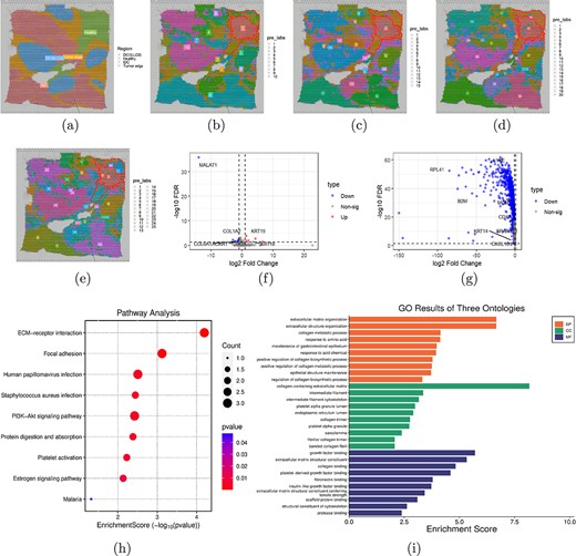
Decipher the progressive lesion area of breast cancer. (a) Visualization of four morphologies included in the manually annotated 20 domains. (b-e) Visualizations of spatial domains identified by TGR-NMF on the first HBRC dataset when the number of spatial domains is set to 10, 15, 20, and 25, respectively. (f) Volcano plot of DEGs between the absolute healthy region and the progressive lesion area. (g) Volcano plot of DEGs between the progressive lesion area and its surrounding cancerous regions. (h) Bubble plot of KEGG pathway analysis. The larger the bubble, the more genes are involved, and the redder the color, the more significant the enrichment. (i) Enrichment analysis results of BP, CC, and MF.
We specifically focused on these DEGs and their biological functions detected between the absolute healthy region and the progressive lesion area. A total of 10 upregulated and 5 downregulated genes were detected under the conditions of |$|log2FoldChange|\geq 0.8$| and |$FDR<0.05$|. The volcano plot of these DEGs was presented in Fig. 5(f). It was worth noting that some genes have been previously identified as key regulators in breast cancer. For example, ACKR1 exhibited a downregulation trend in the progressive lesion area, which may lead to an imbalance in chemokine regulation within the tumor microenvironment. This imbalance could weaken the infiltration and activity of immune cells, allowing tumor cells to evade detection and clearance by the immune system, thereby promoting the progress of breast cancer [39]. The downregulation of COL1A2 reduced the generation of collagen fibers and weakened the integrity of the extracellular matrix, thereby reducing the tissue’s barrier function against tumor cell invasion and accelerating the progress of breast cancer [40]. Additionally, high expression of KRT19 in the progressive lesion area was typically associated with poor breast cancer prognosis and may serve as a potential marker of tumor deterioration [41]. These results indicated that the progressive lesion area contains genes that promoted breast cancer cell growth.
To further validate the progressive lesion area as a transitional zone between the absolute healthy region and the breast tumor edge, we also conducted DEA between the progressive lesion area and its surrounding cancerous regions. As a result, 2926 downregulated genes were detected, as illustrated in Fig. 5(g). Previous studies have shown that the reduced expression of KRT14 can significantly reduce the invasiveness of tumor cells, thereby reducing the risk of metastasis of breast cancer [42]. Additionally, the downregulation of LY6E reduced the expression of VEGFA and PDGFB by decreasing the activation of HIF-1. This process inhibited the PI3K-Akt pathway, thereby reducing tumor angiogenesis in breast cancer [43]. The low expression of CD47 reduced the immune escape signal of tumor cells to macrophages, making tumor cells easier to be recognized and swallowed by macrophages, thus inhibiting the progression of breast cancer [44]. These results indicated that breast cancer suppressor genes were also active in the progressive lesion area. In summary, our results provided strong evidence for the existence of a progressive lesion area as an intermediate stage between the absolute healthy region and the breast tumor edge.
Gene enrichment analysis
Based on the DEGs identified between the progressive lesion area and absolute health region, we conducted KEGG pathway enrichment analysis and GO enrichment analysis. The enrichment scores and names of the various biological pathways were presented in Fig. 5(h), while the genes involved in these pathways were shown in Supplementary Fig. S2. It was worth noting that the ECM-receptor interaction pathway exhibited the highest enrichment score and the most significant p-value. Previous studies have shown that this pathway played a critical role in the progression of breast cancer by mediating interactions between extracellular matrix and cells, thereby affecting tumor cell adhesion, migration, and signal transduction [45]. Additionally, significant enrichment of some other pathways related to breast cancer was also observed. For example, the activation of the PI3K-Akt signal pathway was usually caused by PIK3CA gene mutation or PTEN inactivation, leading to excessive proliferation of breast cancer cells and resistance to apoptotic signals [46]. In estrogen receptor positive (ER+) breast cancer, aberrant activation of the Estrogen signal pathway was a key driver of tumor cell proliferation [47]. These results indicated that the DEGs identified in the progressive lesion area were involved in pathways critical to breast cancer development.
GO includes three main ontologies: biological processes (BP), cellular components (CC), and molecular functions (MF). Figure 5(j) showed the top 10 GO terms with the highest degree of enrichment in each ontology type. The horizontal axis represents the enrichment score, and the vertical axis represents the functional description of the GO item. It was shown that the important GO terms related to BP were mainly enriched in extracellular matrix organization (GO: 0030198, |$p$| = 2.1132E-07), extracellular structure organization (GO: 0043062, |$p$| = 2.1449E-07), and collagen metabolic process (GO: 0032963, |$p$| = 7.2583E-05). At the same time, collagen-containing extracellular matrix (GO: 0062023, |$p$| = 6.7682E-09), intermediate filament (GO: 0005882, |$p$| = 0.0004), and intermediate filament cytoskeleton (GO: 0045111, |$p$| = 0.0007) were significantly enriched in the CC ontology. Similarly, GO terms significantly enriched in the MF ontology included growth factor binding (GO: 0019838, |$p$| = 1.9589E-06), extracellular matrix structural constituent (GO: 0005201, |$p$| = 4.651E-06), and collagen binding (GO: 0005518, |$p$| = 1.479E-05).
Cell communication analysis
Cell communication analysis was conducted to explore the impact of different spatial domains on breast cancer development. The number and strength of interaction between various clusters were shown in circular plots in Fig. 6(a) and (b), respectively. It was observed that the communication network between different clusters was extremely complex, which also confirmed the high heterogeneity within the tumor. To more clearly demonstrate the number and strength of interaction between different clusters, heat maps were generated, as shown in Fig. 6(c) and (d). The results indicated that extensive interactions occur between most clusters, particularly clusters 14, 17, and 13, which may play pivotal roles in tumor growth, invasion, and drug resistance. In contrast, clusters 19, 9, and 16 exhibited relatively fewer and weaker interactions with other clusters. These results emphasized the key role of specific spatial domains in breast cancer progression and suggested that targeted therapeutic interventions against these domains could be of significant importance in tumor treatment.
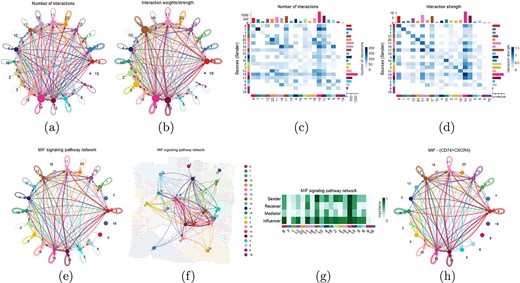
Cell communication analysis. (a) Circle plots of the number of interaction between different clusters. The colors of the nodes represent different clusters. The size of a node is directly proportional to the number of spots in cluster. The arrows point from the source to the target and the color of the edges is consistent with the signal source. (b) Circle plots of the weights/strength of interaction between different clusters. The width of the edges represents the communication probability. (c) Heat map of the number of interaction between different clusters. (d) Heat map of the weights/strength of interaction between different clusters. (e) MIF signal pathway network. (f) Visualization of MIF signal pathway network mapped on spatial transcriptome slice. (g) The centrality scores of the main senders, receivers, mediators, and influencers in the MIF signal pathway network. (h) Circle plot of the number of communications between receptor CD74 and ligand CXCR4 in the MIF signal pathway network.
In the cell-cell communication network, several key signal pathways were identified, including MIF, MK, COMPLEX, SPP1, GALECTIN, CXCL, etc. We focused particularly on the interactions between clusters within the MIF signal pathway, with the network visualization presented in Fig. 6(e). In this network plot, thicker lines represent stronger signal transduction, while clusters with more connections may serve as crucial regulators within the tumor microenvironment. The visualization showed that the MIF signal pathway was particularly active in clusters 14, 17, and 13. Furthermore, the interaction network of the MIF signal pathway was mapped onto spatial transcriptome slices to demonstrate the specific position and distribution of this signal pathway in tissue slices, as shown in Fig. 6(f). To quantitatively analyze the complex cell-cell communication network, we calculated centrality scores of the main senders, receivers, mediators, and influencers in the MIF signal pathway network, which were visualized in Fig. 6(g). The results indicated that clusters 14, 17, and 13 play critical roles in mediating the MIF signal pathway. By calculating the contribution of each receptor-ligand pair in the MIF signal pathway, it was found that MIF-(CD74+CXCR4) contributes most significantly to this pathway. Therefore, we visualized the cell-cell communication mediated by MIF-(CD74+CXCR4), as shown in Fig. 6(h). The figure showed the interaction between ligand CXCR4 and receptor CD74 in the MIF signal pathway, highlighting the importance of this receptor-ligand pair in intercellular signal.
Discussion
To verify that the proposed unitization strategy can effectively handle dropout events, we compared three traditional preprocessing strategies. The first strategy involved eliminating genes with expression values of 0 in more than 80% of the spots. Under this strategy, the ARI and GSCA of the model are 0.2478 and 0.3681, respectively. The second strategy entailed identifying the nearest neighbors of a spot based on spatial coordinate information when a gene had an expression value of 0 in less than 20% of the spots, and then replacing the 0 values with the average expression values of these neighbors. By using this strategy, the ARI and GSCA of the model are 0.2452 and 0.3420, respectively. The third strategy is to simultaneously delete and interpolate genes by combining the first two strategies. Under this strategy, the ARI and GSCA of the model are 0.2417 and 0.3483, respectively. The experimental results indicated that simply deleting genes might have led to the loss of valuable information, while interpolation might have introduced new uncertainties, thereby reducing model performance. Consequently, we proposed a unitization strategy that can fully utilize all the information in the gene expression count data.
The non-negative matrix factorization technique transformed gene expression data into weighted linear combinations of gene features to extract representative gene patterns [32, 48]. The non-negative constraint ensured that the contributions of gene features were positively accumulated, thus avoiding the problem of positive and negative cancellations [49]. This property was consistent with the biological fact that gene expression levels were usually non-negative values, which made the method biologically interpretable. In addition, the gene features produced by this method typically exhibited sparsity, meaning that each feature predominantly depended on a small number of gene expression values. This sparsity not only helped capture key biological patterns, but also effectively reduced noise interference.
In this study, we conducted spatial domain identification experiments on the first HBRC dataset by using Spearman correlation instead of heat kernel weighting. The model achieved an ARI of 0.4822 and a GSCA of 0.5434. The results indicate that the use of Spearman correlation does not enhance model performance compared to the proposed method. This is attributed to the fact that Spearman correlation mainly relies on rank-order relations and cannot fully capture the spatial relevance of expression patterns between spots. The selection of heat kernel weighting for gene expression matrix is to smoothly adjust weights and emphasize the influence between closer spots. From a mathematical perspective, cosine similarity measures the similarity between spots by calculating the angle between two spot position vectors. This method can effectively eliminate the influence of vector length, making the calculation of similarity more focused on the similarity in the vector direction. From a biological perspective, we are more concerned with the relative spatial relationship between different spots rather than their absolute positions when dealing with the spot position coordinate matrix.
In addition, we also adopted a combination of two gene expression neighbors and one spatial location neighbor for identifying the spatial domain of breast cancer. The ARI of the model is 0.5006, and the GSCA is 0.5587. The reason for the poor performance of this model is that more gene expression neighbors may introduce redundant information, making the model learning process more complex. The configuration of selecting one gene expression neighborhood and two spatial position neighborhoods in the proposed model is mainly based on the emphasis on spatial features.
The specific parameter settings of TGR-NMF on the first HBRC dataset were as follows. The scale parameter |$\sigma $| was set to 1. The regularization parameter |$\alpha $| was set to 40 to control the complexity of the model and prevent overfitting. The weight parameters |$\mu _{1}$|, |$\mu _{2}$|, and |$\mu _{3}$| were respectively set to 0.8, 0.19, and 0.01 to balance the contributions of different graph structures to the model. The number of gene expression neighbors |$K_{1}$| and spatial position neighbors |$K_{2}$| were respectively set to 30 and 9 to optimize the capture of local information. The dimension |$k$| in low-dimensional representation was set to 1190 to ensure that sufficient information was retained after dimensionality reduction. In Algorithm 1, minimum error |$\varepsilon $| and maximum number of iterations |$MI$| were set to 0.05 and 500, respectively.
In this paper, TGR-NMF has been presented to decipher spatial domains in breast cancer spatial transcriptomics. It is important that a progressive lesion area that can reveal the progression of breast cancer was uncovered and some pathogenic genes related to breast cancer in this region were identified, including ACKR1, COL1A2, KRT19, etc. Moreover, key signal pathways, such as ECM receiver interaction, PI3K-Akt signal pathway, were also detected. Compared with Seurat, Mclust, BayesSpace, Giotto, SpaGCN, SEDR, and STAGATE, TGR-NMF can decompose spatial transcriptomic data into low-dimensional interpretable combinations of gene features while effectively handling dropout events.
An interesting progressive lesion area (the transition zone between the healthy region and the breast tumor edge) was uncovered through heterogeneity analysis. Further, four biological analyses revealed key genes and pathways associated with breast cancer within the progressive lesion area.
A unitization strategy was proposed to mitigate the impact of dropout events on the computational process, enabling the effective utilization of the complete gene expression count data without the need for deletion or interpolation.
TGR-NMF was constructed by integrating one gene expression neighbor topology and two spatial position neighbor topologies, which can provide an interpretable low-dimensional representation of spatial transcriptomic data.
TGR-NMF achieved high ARI and GSCA in identifying spatial domains in breast cancer spatial transcriptomics, outperforming seven classical methods. Ablation analysis confirmed the effectiveness of the dropout processing strategy and the three graph regularization terms.
Acknowledgement
The author expresses gratitude for the support provided by the high performance computing center of Henan Normal University.
Funding
This work was supported by the National Natural Science Foundation of China [grant numbers 61203293], the Scientific and Technological Project of Henan Province [grant numbers 242102211023].
Code and data availability
Codes and datasets for TGR-NMF are freely available in the GitHub repository (https://github.com/xiangshanxs/TGR-NMF). All datasets used in this paper are published datasets available for download. The first HBRC spatial transcriptomic dataset is collected from the 10|$\times $| Genomics website at https://www.10xgenomics.com/resources/datasets/human-breast-cancer-block-a-section-1-1-standard-1-1-0. The gold standard of the first HBRC dataset is accessible at https://github.com/JinmiaoChenLab/SEDR_analyses/blob/master/data/BRCA1/metadata.tsv. The second HBRC spatial transcriptomic dataset is downloaded from https://zenodo.org/records/4739739.
Author contributions
Juntao Li designed this study. Shan Xiang and Dongqing Wei collected and preprocessed the data. Juntao Li, Shan Xiang, and Dongqing Wei implemented the experiments and analysis. Juntao Li and Shan Xiang wrote the manuscript. All authors have read and approved the final manuscript.
