


Abstract
Single cell RNA sequencing (scRNA-seq) technique enables the transcriptome profiling of hundreds to ten thousands of cells at the unprecedented individual level and provides new insights to study cell heterogeneity. However, its advantages are hampered by dropout events. To address this problem, we propose a Blockwise Accelerated Non-negative Matrix Factorization framework with Structural network constraints (BANMF-S) to impute those technical zeros.
BANMF-S constructs a gene-gene similarity network to integrate prior information from the external PPI network by the Triadic Closure Principle and a cell-cell similarity network to capture the neighborhood structure and temporal information through a Minimum-Spanning Tree. By collaboratively employing these two networks as regularizations, BANMF-S encourages the coherence of similar gene and cell pairs in the latent space, enhancing the potential to recover the underlying features. Besides, BANMF-S adopts a blocklization strategy to solve the traditional NMF problem through distributed Stochastic Gradient Descent method in a parallel way to accelerate the optimization. Numerical experiments on simulations and real datasets verify that BANMF-S can improve the accuracy of downstream clustering and pseudo-trajectory inference, and its performance is superior to seven state-of-the-art algorithms.
All data used in this work are downloaded from publicly available data sources, and their corresponding accession numbers or source URLs are provided in Supplementary File Section 5.1 Dataset Information. The source codes are publicly available in Github repository https://github.com/jiayingzhao/BANMF-S.
Introduction
The improvements in RNA measurement resolution have significantly transformed genomic studies [1]. Contrary to bulk RNA-seq technique, where gene expressions are quantified by the average transcript counts across the ensemble of samples [2], scRNA-seq technique enables the transcriptome profiling of hundreds to ten thousands of cells at the unprecedented individual level [3]. Being able to characterize transcriptional variants in heterogeneous populations, scRNA-seq technique provides new insights to study transcriptional dynamics [4], to explore the changes in cell states [5], to identify transitional cell states [6], and to dissect cell subpopulations [7].
However, the advantages of scRNA-seq data are hampered by its substantial sparsity. The phenomena of having excessive zeros in scRNA-seq data are referred to as dropout events in the context of scRNA-seq data analysis [8]. Those zeros mainly come from two sources. First, a proportion of them, known as “true zeros,” comes from biological fluctuations. For example, a gene may not express RNA in the sample due to changes of external micro-environments. As cells exhibit heterogeneity, some genes may have low or even no expression in specific cell types, cell states, or at special stage of a cell cycle. Second, other zeros are caused by technical reasons, and some genes may be expressed but not captured due to technical limitations during the reverse transcriptional process, such as the limited transcript detection rate and the low sequencing depths. For instance, droplet-based protocols such as Drop-Seq and 10x Genomics protocols are only able to cover 1000 to 200 000 reads per cell [9]. Since most downstream analyses are based on computations on the expression matrix, the extensive technical dropouts may be detrimental to downstream analyses such as clustering and trajectory inference and introduce false discoveries.
Several methods have been proposed to deal with the presence of dropout events [10], which address the problem mainly from three perspectives [11]. The first category explores the vertical structure of the underlying data. Those imputation models focus on exploiting gene–gene similarity to estimate the possible locations of technique zeros and recover their values, such as SAVER [12]. The second category explores the horizontal structure of the expression matrix. Those models assume that similar cells hold similar expression level and then recover missing values from a cell–cell perspective. Typical algorithms include MAGIC [13], scImpute [14], DrImpute [15], bayNorm [16], and scRMD [17]. The third category explores the diagonal structure of the expression matrix, and they assume that the matrix should follow a low-rank structure and typically adopt matrix-factorization based models to capture linear relationships in the latent space. Those methods project the observed expression data into a low-dimensional space and recover the expression values through low-rank matrices multiplication, for instance, ALRA [18]. Besides, deep-learning based methods are capable of capturing the non-linear relationship between cells and try to recover the expression levels through different decoders. AutoImpute uses an auto-encoder to estimate a latent space that learns the inherent distribution of the scRNA-data, and it can impute those dropout events and preserve the true zeros at maximal level [19]. scMultiGAN imputes the cell-type specific dropout based on multiple GANs [20]. Although existing methods have demonstrated some strengths in imputation, there is still room for improvement. First of all, the first and second classes of methods fail to jointly learn the gene and cell similarity; therefore, they may tend to favor certain situations where the observed gene/cell expressions are consistent and under-perform in other cases. Besides, the third class fails to incorporate gene and cell similarity so that the underlying structure may not be fully utilized. Secondly, the existing methods do not fully integrate prior information. For example, STRING is a comprehensive database for Protein–Protein Interaction (PPI), providing extensive information about functional associations between proteins, such as physical interactions, co-expression, and shared pathways [21], foreshadowing gene–gene similarity. However, none of the above-mentioned methods takes full advantage of those prior information. Thirdly, contemporary methods mainly characterize cell (or gene) similarity simply by calculating the Euclidean distance between their low-dimensional expression representations, and this may fail to further exploit the high-order relationships. Fourthly, existing methods fail to assimilate temporal information, which may overlook the information in the developmental progressions from samples.
To fully address these problems, we try to incorporate both gene similarity and cell similarity to impute scRNA-seq data. The proposed method is called Blockwise Accelerated Non-negative Matrix Factorization imputation with Structural network constraints, shorted as BANMF-S. In a nutshell, BANMF-S is based on the framework of non-negative matrix factorization; it constructs a gene–gene similarity network to integrate prior information from the external PPI network by the Triadic Closure Principle (TCP) [22] and a cell–cell similarity network to capture the neighborhood structure and temporal information through a Minimum-Spanning Tree (MST), so as to assimilate internal information from observations. By collaboratively employing these two networks as regularization, BANMF-S encourages the coherence of similar gene and cell pairs in the latent space, enhancing the potential to recover the underlying features, which are demonstrated by simulation studies in Section 3. Downstream experiments on clustering and lineage reconstruction validate that BANMF-S outperforms other seven state-of-the-art methods in both simulated and real cases (see Results section). To tackle the large-scale problem in scRNA-seq data, we applied a stratified matrix blocklization strategy, which enables the optimization process through distributed Stochastic Gradient Descent (SGD) method in a parallel way. The computational efficiency and scalability of BANMF-S are shown in Results section.
Materials and methods
Problem formulation
Given the raw counts |$\tilde{X}\in \mathbb{R}^{m\times n}$| from scRNA-seq experiments for |$m$| cells and |$n$| genes, we normalized each library (row) to |$10^{4}$| counts per cell, added one pseudocount, and performed |$\log _{2}$| transformation (see a detailed illustration in Supplementary File Section 7.2 Data Preprocessing). The processed matrix is denoted as |$X_{0}$| and |$X$| is used to denote the genuine expression matrix (without technical noise). The relationship of |$X$| and |$X_{0}$| is obtained by a binary mask operator |$M$| (|$[M]_{ij} = 0$|, if |$[X_{0}]_{ij} = 0$|) as Eq. (1) suggests where |$\circ $| is the Hadamard product operator,
Previous argument states that only a few biophysical functions trigger the functioning transcription factors [23], indicating that the generated expression matrix lies in a low-dimensional space. We assumed that the genuine matrix can be factorized into the product of two low-dimensional nonnegative matrices, that is, |$X=WH$|, where |$W\in \mathbb{R}^{m\times p}$| and |$H\in \mathbb{R}^{p\times n}$| with |$ p\ll m,n$|. Here, |$W$| represents the low-dimensional cell matrix and |$H$| represents the low-dimensional gene matrix. The NMF was then obtained by solving the following optimization problem:
where |$||\cdot ||_{F}$| is the Frobenius norm and ‘|$\geq 0$|’ indicates the matrices are non-negative. However, the non-negativity constraints in Eq. (2) cannot guarantee the coherence of gene or cell similarity, and it fails to exploit the underlying gene and cell structure, which may result in the failure of |$W$| and |$H$| to recover biological variants. To take into account these concerns, we proposed a structural network constraints regularized framework to incorporate gene and cell similarities, and they are illustrated as follows.
Gene similarity
We integrated the prior knowledge of a PPI network to ensure the consistency of similar genes. First, a PPI network was obtained from the STRING database through R package STRINGdb version 2.10.1. Then, we employed TCP to quantify the structural similarity of proteins from their physical and functional interactions provided by PPI [21]. Since the structure of a protein is determined by its gene sequence [24], we use the computed protein structural similarity to quantify the similarity of gene pairs. We call it gene high-order similarity for two reasons: firstly, the gene similarity is quantified by its downstream products rather than the direct sequences. On the other hand, the similarity is characterized by the higher-order relationships between nodes rather than the direct interactions. Rooted in social network analysis, TCP asserts that two individuals are more likely to know each other if they have more common friends. Accordingly, we assumed that two proteins are more likely to be structurally similar if they share more common neighbors in the PPI network. This can be explained from a structural perspective illustrated in Fig. 1c: if two proteins |$P_{1}$| and |$P_{2}$| share multiple interaction partners, then they may have similar interaction interfaces, which further reflects in the similarity of gene pairs.
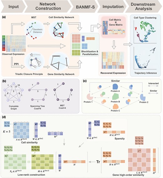
BANMF-S schematic: (a) BANMF-S mainly contains five steps; a raw cell-by-gene expression matrix is required as input, then in the network construction step, BANMF-S obtains gene similarity network by integrating PPI network from STRING database based on TCP and computes cell similarity network from the reciprocal of geodesic distance of the MST on the complete graph generated by the first 50 principal components of the input matrix, and the core module of BANMF-S solves the constrained NMF problem in parallelization by adopting a blocklization strategy; the imputation is completed by recovering expression levels from the outputs of gene and cell matrices, which can be used in downstream analysis studies, such as clustering and trajectory inference; (b) an example of MST on a 5-node complete graph; (c) an illustration for TCP that demonstrates the pair who shares a large amount interacted proteins are structurally similar; (d) an example of blocklization strategy for a 10-by-15 expression matrix where |$K=5$|.
Hence, we quantified the similarity of Gene |$i$| and Gene |$j$| by the ratio of shared neighbors of their corresponding proteins |$P_{i}$| and |$P_{j}$|. To be precise, let |$S$| be the adjacent matrix of the gene similarity network, then its (|$i$|,|$j$|)th entry can be calculated by the Jaccard Index as shown below
where |$N_{P_{i}}$| is the set of neighbors of the protein |$P_{i}$|, |$i=1,2$|. Then, we added the graph regularization |$Tr(HLH^{T})$| [25] to the objective function to capture the gene similarity structure where |$L: =\text{diag}(S \cdot \mathbf{1}) - S$| is the Laplacian to |$S$| and |$\mathbf{1}$| is the constant one vector. The geometric interpretation of the graph regularization |$Tr(HLH^{T})$| is given in Supplementary File Section 1.
Cell similarity
We then incorporated the underlying knowledge of temporal information in cell development to absorb cell similarity. Firstly, we applied dimension reduction to the observed expression matrix |$X_{0}$| by using Principal Component Analysis. We selected top 50 principal components, the resulting matrix was denoted as |$X_{PC}\in \mathbb{R}^{m\times 50}$|. Then, a fully connected undirected graph |$G(V, E)$| was constructed from |$X_{PC}$|, where |$V =\{v_{1}, v_{2}, \cdots , v_{m}\}$|, and |$E=\{e_{ij}, i, j \in \{1,2,\cdots , m\}\}$|. Node |$v_{i}$| represents the |$i$|th cell, and |$e_{ij}$| denotes the edge connecting cell |$i$| and cell |$j$| of which the weight |$\omega _{ij}$| can be calculated as the Euclidean distance between the |$i$|th row and the |$j$|th row of |$X_{PC}$|. Secondly, we computed the minimum spanning tree of |$G(V, E)$| and denoted it by |$T$|. Contrary to previous methods [13] where Euclidean distance was directly used to characterize affinity, we used the reciprocal of the geodesic distance of |$T$| to measure the similarity between cells. Specifically, let |$A$| be the adjacency matrix of cell similarity network, then |$A_{ij}$| was computed by
where ShortestPath|$(T(i,j))$| is the shortest path between |$i$| and |$j$| on |$T$| and length(|$\cdot $|) indicates the total Euclidean length of that path. For example, as shown in Fig 1b, the left subgraph is fully connected and undirected, each edge measures the distance between its corresponding two nodes, the middle subgraph gives a possible spanning tree, and the right subgraph shows the minimum spanning tree. Following above instructions, similarity score for the unconnected pair of nodes in the upper right should be |$1/4$|, since the shortest length between them is |$4$|. Notably, we chose this quantification for two reasons. First, Costa et al. [26] proposed that MST-based matrix is more capable of preserving the local invariance property than Euclidean-based distance on the approximation of local neighborhood structure. Second, MST is intrinsically related to cell differentiation since loads of trajectory inference methods are based on MST spanned on the reduced dimensional observation [27]. Hence, Eq. (4) captures the ordering of cells along the developmental progression, assimilating temporal information.
In this paper, we adopted the regularization term |$\|A - WW^{T}\|_{F}^{2}$| to ensure that similar cells would show similar expression patterns. This regularization term was initially added to address the graph clustering problem in [28], and here, we used it to inherit cell neighborhood structure from cell similarity network. Besides, the cell structural regularization |$\|A - WW^{T}\|_{F}^{2}$| has intrinsic relationships with graph regularization term |$Tr(W\tilde{L}W^{T})$| (See Supplementary File Section 1); here |$\tilde{L}$| refers to the normalized graph Laplacian for the cell similarity network.
Finally, we added the terms |$\|H\|_{F}^{2}$| and |$\|W\|_{F}^{2}$| to ensure sparsity. To wrap up, our objective function becomes
where |$\alpha _{1}, \alpha _{2}, \gamma _{1}, and \gamma _{1}$| are hyper-parameters.
Blockwise acceleration
When optimizing the objective function (5), we need to compute the following gradients:
The total computational costs would be |$\mathcal{O}(mnp+m^{2} p+n^{2} p)$| for each iteration. Since sizes of gene similarity network are usually very huge, the traditional implementation of gradient descent method could be computationally expensive and it is not ideal for recovering large-scale expression profiles. We considered employing a blocklization strategy to accelerate the implementation through a distributed version of SGD.
In the distributed SGD, original data matrix was firstly divided into blocks. Let |$K$| be the prescribed number of splits, let |$ m_{d} = \lfloor \frac{m}{K} \rfloor $| and |$n_{d} = \lfloor \frac{n}{K} \rfloor $|. We divided |$X_{0}$|, |$A$|, |$M$|, |$W$|, |$H$| and |$L$| into |$K^{2}$| blocks of various sizes, see a toy example in Figure 1(d), detailed illustrations were provided in the Supplementary File Section 2. Superscripts are used to denote blocks, for instance, let |$A^{ij}$| represent the |$j$|th column split at |$i$|th row split in |$A$|. Afterward, the traditional optimization is accelerated in parallelization by simultaneously updating interchangeable blocks over multiple processes. In more details, at the |$t$|th iteration, quadruples of indices |$U^{t}:=\{(i_{1}^{t}, j_{1}^{t}, r_{1}^{t}, s_{1}^{t}),(i_{2}^{t}, j_{2}^{t}, r_{2}^{t}, s_{2}^{t}),\cdots \}$| were first randomly generated. Then, the corresponding quadruples of blocks |$\{(W^{i_{1}^{t}}, W^{j_{1}^{t}}, H^{r_{1}^{t}}, H^{s_{1}^{t}}),(W^{i_{2}^{t}}, W^{j_{2}^{t}}, H^{r_{2}^{t}}, H^{s_{2}^{t}}),\cdots \}$| were separately updated in various processes to minimize the objective function (5) by gradient descent. Take |$(i,j,r,s)\in U^{t}$| for instance, in the parallelized process of its own, |$W^{i}$| and |$W^{j}$| were updated to approximate |$A^{ij}$|, similarly, |$H^{r}$| and |$H^{s}$| were updated to minimize |$Tr(H^{r} L^{rs} (H^{s})^{T})$|. Also, |$W^{i}$| (or |$W^{j}$|) and |$H^{r}$| (or |$H^{s}$|) were updated to approximate |$X_{0}^{ir}$| (or |$X_{0}^{js}$|,|$X_{0}^{is}$|,|$X_{0}^{jr}$|, respectively). Then, the overall loss function can be rewritten as the sum of blockwise loss
where
To ensure the independence of each process, interchangeability [29] of the index quadruple set |$U^{t}$| should be maintained so that the optimization of |$(W^{i}, W^{j}, H^{r}, H^{s})$| would not affect another pairs (see Supplementary File Section 3 for details). For each subprocess, let |$\theta ^{i,j,r,s}=\{W^{i}, W^{j}, H^{r}, H^{s}\}$|, then |$\theta ^{i,j,r,s}$| can be updated through gradient descent, where
Here, |$\eta _{t}$| is the step-size at the |$t$|th iteration. The algorithm for solving Equation (5) is summarized in Algorithm 1 in Supplementary File Section 4.
Results
We conducted various simulated and real experiments to test the performance of BANMF-S, where eight scRNA-seq datasets and one bulk RNA-seq dataset were used (see summary Supplementary File Section 7.1 Datasets), and chose seven methods (see summary and a brief illustration in Supplementary Table 2 and Supplementary Section 7 Experiments) for comparison. For all the methods, we followed their online vignettes and adopted default parameters. For BANMF-S, all parameters are provided in Supplementary Table 10 (see Supplementary Section 12 for details).
BANMF-S outperforms state-of-the-art algorithms in simulations
We generated simulations from PBMC dataset to investigate the performance of BANMF-S in recovering the true biological signals. Since the genuine dropout locations are usually unknown, we considered two simulation setups to manually curate the ground truth and then randomly removed several captured entries and regarded them as missing values. The results were assessed from two perspectives (RMSE and cell-wise correlation, see Supplementary File Section 7.4 Evaluation).
In the first simulation approach, the ground truth was created by selecting high-quality genes and samples with large coverage from the PBMC dataset, and this generated a dense matrix. The filtered PBMC dataset contains |$11.75\%$| non-zero entries. By retaining genes with capture rates in the first half quantile and cells with library depths in the first |$80\%$| quantile, we obtained a reference matrix of 1578 cells and 4586 genes with |$22.01\%$| non-zero values, whose entries are treated as true expression. Afterward, we added additional noises on the curated matrix through a Binomial down-sampling procedure. To be specific, we randomly removed non-zero reads by Binomial distribution |$B(n, p_{i})$|; |$p_{i}$| was the dropout rate for |$i$|th gene. To study the imputation results under various dropout rates, we perturbed |$p_{i}$| at levels |$30\%, 35\%, 40\%, 45\%, 50\%, 55\%$|, and |$60\%$|, to ensure the density of the simulated matrices was within |$0.75 \sim 1.35$| of the original matrix’s density (see Supplementary Table 3). Then, we evaluated the similarity of imputed matrices and the 7 genuine matrices by RMSE and cell-wise correlation. The RMSE values are given in Supplementary Table 5, and the relative ranks of RMSE within each simulated datasets are given in the simulation 1 in Fig. 2a. The results of RMSE demonstrate that BANMF-S and ALRA are the best two methods in simulation 1, while the model-based methods bayNorm and SAVER lack the capability to recover overall expression level accurately. Also, the results indicate that BANMF-S performs better in sparse cases (downrate |$50, 55$|, and |$60$|). Figure 2b provides the violin plots of cell-wise correlation for each cell types in simulation 1, which shows that BANMF-S and MAGIC are the best two methods to recover sample-level biological similarity. Besides, the violin plots demonstrate that BANMF-S, MAGIC, scImpute, and scRMD are more consistent with low variances.
In the second approach, bulk immune cell RNA-seq data (GSE74246) was used to curate ground truth. The bulk RNA-seq dataset contains four samples for each cell types of B cell, CD4+ T cell, CD8+ T cell, NK cell, and Monocyte. It can be regarded as well-defined expression references of PBMC in our study. In simulation 2, we used multinomial distribution to simulate the ground truth, where the bulk profiles were used for gene expression distributions and the single cell data library sizes were used as true library depths. We used Monocyte as an example to illustrate the simulation. Denote the gene reads proportion in bulk Monocyte data as |$\textbf{p}_{i}$|, where |$i$| indicates samples, |$i=1,\cdots , 4$|. The library lengths of Monocytes in single cell RNA-seq dataset are |$n_{c}$|, where |$c=1, \cdots , \mathcal{C}_{monocyte}$|, and |$\mathcal{C}_{monocyte}$| is the number of Monocyte cells. Then, we generated the ground truth expression profile for |$c$|th cell as
and we obtained |$4\times \mathcal{C}_{monocyte}$| artificial Monocyte cell expression profiles. Then, we applied Binomial down-sampling procedure to obtain noisy matrices similar to simulation 1 and the down-sampling rates for each cell types are given in Supplementary Table 4. Figure 2a shows that BANMF-S performs best in B cell (RMSE: 1.1385), CD8+ T cell (RMSE: 1.1974), and Monocyte (RMSE: 1.0603). Figure 2c provides the violin plots for the five datasets in simulation 2, which shows that BANMF-S and MAGIC are the best two methods to recover sample-level biological similarity.
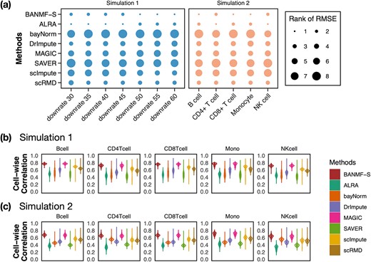
Simulation results: (a) rank of RMSE; (b) violin plots of cell-wise correlation for five cell types in simulation 1; (c) violin plots of cell-wise correlation for five cell types in simulation 2.
BANMF-S improves the performance of cell type clustering
Clustering serves as an essential step in scRNA-seq data analysis, aiming to partition individuals within a heterogeneous population into distinct groups. A good imputation method is supposed to improve the outcomes of clustering, which helps gain valuable insights into the inherent structure and patterns of the expression profile. We assessed the impact of our method on seven real datasets (see Supplementary File Section 7.1 for details). After processing datasets and applying imputation methods as suggested by Section 7 Experiments in Supplementary File, we first explored the results of Pollen by UMAP, a nonlinear dimensionality reduction technique that helps visualize high-dimensional data. UMAP results for other datasets are provided in Supplementary File Section 9. As is shown in Fig. 3a, all methods except bayNorm (5 cliques) and scRMD (5 cliques) give a more consistent profiling of the number of clusters in the latent space than no imputation (Raw: 5, BANMF-S: 9, ALRA: 11, DrImpute: 6, MAGIC: 9, SAVER: 8, scImpute: 8), improving the characterization of the heterogeneous composition. Among them, BANMF-S outperforms ALRA and MAGIC by accurately gathering Kera and K562 cells. Moreover, BANMF-S outperforms SAVER, scImpute, and DrImpute by indentifying more cliques.

Clustering Evaluation: (a) UMAP plot for Pollen dataset; (b) clustering accuracy evaluation (ARI and NMI) results.
Then, we performed |$k$|-means clustering (R stats package, version 4.0.4), an unsupervised clustering method, on the top 10 principal components of the imputed and observed data, where we used true cell type number as the number of clusters for parameter centers. We also considered the clustering results on cell matrix |$W$|, results are named by BANMF-S-latent, shown in Fig 3b. The outcomes are evaluated by ARI and NMI (see Supplementary File Section 7.4 Evaluation), where larger values indicate better consistency between inferred clusters and true cell type labels. As is shown in Fig. 3, BANMF-S and BANMF-S-latent demonstrate an overall higher accuracy compared with raw data (denoted by noimp in Fig. 3b), indicating its capability to enhance the performance of downstream clustering analysis. The ARI and NMI values are also recorded in Supplementary Tables 6 and 7. Moreover, we can also conclude from overall ARI and NMI values that BANMF-S and BANMF-S-latent are superior to other 7 imputation methods. Specifically, BANMF-S and BANMF-S-latent achieve the best two places in PBMC and Petropoulos. BANMF-S-latent has the best ARI performance in Pollen (ARI: 0.7473) and Baron_Ms (ARI: 0.5806), indicating that BANMF-S is able to improve the accuracy of identifying subpopulations from tissue and cell line data. As BANMF-S-latent demonstrates the best performance among all methods, we recommend using the our cell matrix outcomes for computational cell annotations in future studies.
BANMF-S improves the performance of pseudotime trajectory reconstruction
Cell lineage reconstruction is a crucial downstream analysis for scRNA-seq data, where computational approaches [30] are utilized to reconstruct the developmental trajectories of samples based on their gene expression profiles. An effective imputation method is expected to enhance the performance of pseudotime trajectory reconstruction by accurately recovering the continuous topological structure of the data.
To evaluate our method, we conducted experiments on two publicly available time-serial scRNA-seq datasets: the Petropoulos [31] and the Scialdone [32] datasets, and compared our results with other seven methods (see Supplementary Table 2) as well as the results on the raw data. Pseudotime labels for all cells were obtained by monocle2 with default parameters, and we then calculated the Pearson and Kendall’s correlation between Pseudotime labels and experimentally recorded time stamps, and used these two correlation scores to evaluate accuracy for each method. Results are presented in Table 1. Visualizations of the inferred trajectories are provided in Supplementary File Section 11. In Petropoulos dataset, BANMF-S exhibits both higher Pearson correlation score (0.9216) and Kendall’s correlation score (0.7868) compared with raw data (0.9018 and 0.7310, respectively). Similarly, in Scialdone dataset, BANMF-S achieves a Pearson correlation score of 0.8621, a Kendall’s correlation score of 0.6432, whereas the score for raw data are 0.7984 and 0.5557, respectively. These results demonstrate that BANMF-S can improve the performance of downstream pseudotime analysis. When compared with other imputation methods, it can be observed that BANMF-S achieves the highest correlation scores among the counterparts for Pearson Correlation. As for Kendall’s rank correlation, BANMF-S obtains the best accuracy (0.7858) in Petropoulos dataset and the third highest accuracy (0.6432) in Scialdone dataset, where the accuracy gaps between BANMF-S, scImpute (0.6542), and SAVER (0.6465) are close and acceptable.
Trajectory correlation
| Dataname | ALRA | bayNorm | BANMF-S | MAGIC | Raw | SAVER | scImpute | scRMD | DrImpute |
|---|---|---|---|---|---|---|---|---|---|
| Petropoulos (Kendall) | 0.6107 | 0.7425 | 0.7868 | 0.7751 | 0.7370 | 0.6985 | 0.7614 | 0.7183 | 0.7615 |
| Scialdone (Kendall) | 0.6368 | 0.5807 | 0.6432 | 0.5548 | 0.5557 | 0.6465 | 0.6542 | 0.6025 | 0.6298 |
| Petropoulos (Pearson) | 0.8248 | 0.9041 | 0.9216 | 0.9187 | 0.9018 | 0.8812 | 0.9131 | 0.8962 | 0.9145 |
| Scialdone (Pearson) | 0.8564 | 0.8384 | 0.8621 | 0.8263 | 0.7984 | 0.8536 | 0.8520 | 0.8546 | 0.8481 |
BANMF-S is an efficient algorithm
In this section, we evaluate the time and memory costs of imputation methods being implemented on an AMD EPYCTM 7742 server (64 CPU Cores; 512GB RAM; 480GB SSD). Starting from here, we use italic font for datasets and telegram font for variables in the source codes of the corresponding methods. We performed cell downsampling and gene downsampling on pbmc10k dataset to assess the computational efficiency at different scales of cells and genes. To be specific, we first selected |$10^{4}$| genes and cells of most reads to obtain cell 10k dataset. Then, we generated cell 1k, 3k, 5k, 7k, 10k datasets by randomly subtracting submatrices of corresponding cell numbers from cell 10k. The gene 1k, 3k, 5k, 7k, 10k datasets could be obtained in a similar gene downsampling way, i.e. by randomly subtracting submatrices of corresponding gene numbers from cell 10k. For BANMF-S, we assumed that the gene and cell similarity networks were known and skipped the network construction step. Computational time (in hour) and memory usage (in GB) were obtained by Slurm command sacct with job accounting field elapsed and MaxRSS. To mitigate the potential impact of systems fluctuations in the execution time, all methods were repeated five times on each dataset and the averaged time and memory records were used for evaluation.
We first assessed the computational efficiency of all methods on large-scale dataset by using the results of cell 10k from Fig. 4a. From the distances of scatter dots to origin, it can be inferred that scImpute, DrImpute, SAVER, and scRMD demonstrate poor performance, while MAGIC, BANMF-S, ALRA, and bayNorm are computationally efficient. Using parallelization, the computational time of BANMF-S (0.1142 h) is close to the fastest methods, the matrix-based method ALRA (0.0650 h) and MAGIC (0.0904 h), indicating the effectiveness of the blocklization strategy. In terms of memory usage, BANMF-S (5.7086 GB) demonstrated significant improvement compared with matrix-based method scRMD (21.8855 GB).
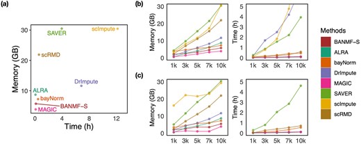
Time and memory usage evaluation: (a) gives the results of cell 10k dataset; (b) time and memory cost for cell sampling datasets; (c) time and memory cost for gene sampling datasets.
Then, we evaluate the scalability of the methods from Figs 4b and c, where we manually scale the |$y$|-axis limits to 30 GB and 5 h to focus on efficient results. The time results of scImpute and DrImpute on gene sampling datasets (Fig. 4c) all exceed 5h since they need to compute cell–cell similarity matrix for |$10^{4}$| cells, showing poor scalability for large-scale cell datasets. Close to the |$x$|-axis, time plots of Fig. 4 b and c show that ALRA, MAGIC, and BANMF-S are the three fastest methods with indistinguishable difference. As for the memory usage, memory plots of Fig. 4b and c indicate that BANMF-S gives an overall outperformance over bayNorm, DrImpute, SAVER, scImpute, and scRMD across all cases. Though BANMF-S requires larger disk memory than ALRA in small datasets (cell 1k, gene 1k), BANMF-S surpasses ALRA in other situations, indicating the scalability and the effectiveness of blocklization. Figure 4b and c shows that MAGIC has less memory usage than BANMF-S in all cases, since BANMF-S requires the storage of gene and cell networks. The resulted memory differences for MAGIC and BANMF-S are acceptable, as the memory outperformance of MAGIC comes at the cost of losing cell and gene information.
The blocklization strategy improves the computational efficiency in two ways. On the one hand, it enables BANMF-S to solve the traditional NMF problem by SGD in parallelization, saving wallclock time for large-scale datasets. On the other hand, it allows BANMF-S to improve computational memory cost by circumventing direct large-scale matrix computations, and therefore, avoids the storage of numerous large-scale intermediate matrices. As is shown in the memory plots in Fig. 4b and c, the slopes for the matrix-based methods, scRMD and ALRA, are larger than BANMF-S. This is because scRMD and ALRA failed to deallocate many intermediate |$m-$|by|$-n$| matrices during optimization. With those redundant variables, scRMD and ALRA may be resource-acceptable for small-scale datasets, but resource-intensive, even detrimental when confronted with large-scale datasets. Back to BANMF-S, our method first restores |$X_{0}, M\in \mathbb{R}^{m\times n}$|, |$A\in \mathbb{R}^{m\times m}$|, and |$L\in \mathbb{R}^{n\times n}$| in the global environment. In the core computational module, rather than the direct manipulation of the |$m-$|by|$-n$| matrix, we tackled matrices of |$\mathcal{O}(m_{d}n_{d})$|. At each iteration, we sampled block quadruples to |$K$| registered pipes (processes in the context of parallelization), where each pipe contained variables of |$\{A^{ij}\in \mathbb{R}^{m_{d}\times m_{d}}, L^{rs}\in \mathbb{R}^{n_{d}\times n_{d}}, W^{i},W^{j}\in \mathbb{R}^{m_{d}\times p}, H^{r},H^{s}\in \mathbb{R}^{p\times n_{d}}, X_{0}^{ir}, X_{0}^{is}, X_{0}^{jr}, X_{0}^{js}, M^{ir}, M^{is}, M^{jr}, M^{js}\in \mathbb{R}^{m_{d}\times n_{d}}\}$| and the derivatives |$\{\nabla _{W^{i}} \tilde{O}, \nabla _{W^{j}} \tilde{O}\in \mathbb{R}^{m_{d}\times p}, \nabla _{H^{r}} \tilde{O}, \nabla _{H^{s}} \tilde{O}\in \mathbb{R}^{K\times n_{d}}\}$|. To sum up all processes, the maximum memory requirement of our computational module can be regarded as |$K\cdot m_{d}n_{d} + K\cdot m_{d}^{2} + K\cdot n_{d}^{2}$|, which demonstrates considerable improvements in terms of memory compared with the whole scale. A detailed illustration is provided in Supplementary File Section 8.
Discussions
In this paper, we propose a novel NMF framework by jointly incorporating the similarity information from external and internal sources, namely that the cell similarity network and the gene similarity network were added as graphical constraints. We integrated STRING database to preserve gene structure for gene matrix and incorporated temporal orders to assimilate the intrinsic information along the biological progression to enhance the cell structure for the cell matrix. Our constrained framework bridges the gap that none of existing methods tackles the dropout problem from a collaborative view of gene and cell similarity while assimilating prior and temporal information. Experiments and downstream analyses on real and simulated data demonstrate the effectiveness of our network constraints. Besides, we made our method scalable by adopting a blocklization strategy, by which we solved the optimization problem in parallelization. By employing BANMF-S on datasets of different scales, we demonstrate that our method is computationally efficient.
There are several possible improvements for future studies. Firstly, the cell similarity network could be constructed through cluster-based MST (cMST) to alleviate the tedious computations for large-scale MST. To be specific, similar to monocle2 [33], we could first perform unsupervised clustering to identify cell states, then construct the “backbone” MST on these centers. Afterward, the temporal orders could be inferred by geometric projections on the cMST. Secondly, with the development of spatial transcriptomics, high-quality spatial information for cells are available and leveraging the spatial similarity of cells should be considered into the construction of cell similarity network. Thirdly, in our work, the gene similarity network is quantified from PPI network only. However, there are other gene information that could be integrated, such as ChIP-Seq data. The way to deal with various sources of prior information still needs further investigation.
Acknowledgements
We extend our sincere gratitude to Yuzhao Wang from Sun Yat-sen University Cancer Center and Anqi Xu from the School of Biomedical Sciences at the University of Hong Kong for their helpful discussions and constructive feedbacks throughout the development of this paper. The computations were performed using research computing facilities offered by Information Technology Services, The University of Hong Kong.
Conflict of interest: None declared.
Funding
This work is supported in part by funds from the National Science Foundation of China (NSFC: #11801434, #12090020, #12090021), Hong Kong Research Grants Council under GRF Grants # 17301519 and # 17309522, and Hung Hing Ying Physical Sciences Research Fund, HKU.
References
