


Abstract
The recent advances of single-cell RNA sequencing (scRNA-seq) have enabled reliable profiling of gene expression at the single-cell level, providing opportunities for accurate inference of gene regulatory networks (GRNs) on scRNA-seq data. Most methods for inferring GRNs suffer from the inability to eliminate transitive interactions or necessitate expensive computational resources. To address these, we present a novel method, termed GMFGRN, for accurate graph neural network (GNN)-based GRN inference from scRNA-seq data. GMFGRN employs GNN for matrix factorization and learns representative embeddings for genes. For transcription factor–gene pairs, it utilizes the learned embeddings to determine whether they interact with each other. The extensive suite of benchmarking experiments encompassing eight static scRNA-seq datasets alongside several state-of-the-art methods demonstrated mean improvements of 1.9 and 2.5% over the runner-up in area under the receiver operating characteristic curve (AUROC) and area under the precision–recall curve (AUPRC). In addition, across four time-series datasets, maximum enhancements of 2.4 and 1.3% in AUROC and AUPRC were observed in comparison to the runner-up. Moreover, GMFGRN requires significantly less training time and memory consumption, with time and memory consumed <10% compared to the second-best method. These findings underscore the substantial potential of GMFGRN in the inference of GRNs. It is publicly available at https://github.com/Lishuoyy/GMFGRN.
INTRODUCTION
Gene regulatory networks (GRNs) refer to the complex interactions among genes that dictate the patterns of gene expression and regulatory processes across diverse conditions. These networks play a pivotal role in cellular differentiation, development and disease progression [1]. Reconstructing GRNs therefore can provide insights into the mechanisms that underlie gene regulation in biological processes, thereby further improving our understanding of the complex interaction between genotype and phenotype in any species. Recent advances in high-throughput sequencing technologies [2] have enabled the acquisition of high-resolution gene expression data at the single-cell level. This single-cell RNA sequencing (scRNA-seq) technique can reveal cellular heterogeneity, transcriptional states and transitions, and capture cell-type-specific features and biological information. Consequently, the inference of GRNs using scRNA-seq data has gained increasing attention in biology and bioinformatics areas [3–6]. However, due to cell heterogeneity [7], cell cycle effects [8] and dropout events [9] in scRNA-seq data, reconstructing GRNs remains a challenging task.
To address these challenges, several methods have been developed to infer GRNs from scRNA-seq data, which can be generally divided into unsupervised [10–24] and supervised methods [3–5, 25–30]. Unsupervised methods mainly include information theory-based methods [10–13, 15, 18, 22], model-based methods [16, 20, 21, 23, 24, 31–34] and machine-learning-based methods [14, 19, 35]. The information theory-based methods encompass various approaches, such as mutual information (MI) [12], Pearson correlation coefficient (PCC) [10, 11], partial information decomposition and context (PIDC) [13] and Normi [22]. By conducting correlation analysis, these methods assume that the strength of the correlation between genes is positively correlated with the likelihood of regulation between them. The model-based approaches involve fitting gene expression profiles to establish a model that accurately describes the relationships between genes and subsequent use of such model to reconstruct GRNs. These methods exhibit high flexibility and scalability, allowing the selection of different models based on the data types and network characteristics. Representative methods include LogBTF [24] and MetaSEM [23]. LogBTF [24] is a Boolean network model that efficiently infers GRNs by combining regularized logistic regression and Boolean threshold functions. MetaSEM [23] employs structural equation model (SEM) to simulate regulatory relationships between genes and utilizes meta-learning to address parameter optimization challenges posed by high-dimensional sparse scRNA-seq data. Some machine-learning-based unsupervised methods have also been published. For example, GENIE3 [19] employs random forest [36] to independently infer the GRN of each gene and takes multiple transcription factors as inputs to fit the expression value of a target gene. The feature importance ranking of the random forest is viewed as the regulatory scores of these transcription factors (TFs) with respect to that target gene. While these unsupervised methods do not require label information, they struggle to effectively handle the noise, dropouts, high sparsity and high dimensionality characteristics of scRNA-seq data. Furthermore, most unsupervised methods are typically applicable only to small datasets, as excessively large datasets may result in ‘endless’ computational time.
Recently, the emergence of deep-learning techniques and the accumulation of ChIP-seq data have been predominantly used in supervised methods for GRN inference. Supervised methods hypothesize that partial gene regulations have been annotated, and subsequently apply machine-learning methods, such as neural networks, to learn the features of regulated genes and their transcription factors. These features are then utilized to predict unknown gene regulatory relationships. In recent years, several methods have been developed for inferring GRNs using deep-learning techniques. Some representative ones include (DGRNS) [25], 3DCEMA [26], (CNNC) [3] and DeepDRIM [4]. DGRNS [25] combines recurrent neural networks for temporal features extraction and convolutional neural networks (CNNs) for spatial features extraction to infer GRNs. 3DCEMA [26] is another deep-learning-based method that categorizes gene expression values into 16 bins representing different expression levels and constructs a 3D co-expression matrix using a third gene to identify regulatory relationships through 3D convolutional neural networks [37]. CNNC [3] transforms the identification of gene regulation into an image classification task by converting the expression values of a pair of genes into a histogram and using a convolutional neural network for classification. However, the performance of CNNC suffers from the issue of transitive interactions. To address this, DeepDRIM [4] considers the information of neighboring genes and transforms TF–gene pairs and neighboring genes into histograms as additional inputs, thereby reducing the occurrence of transitive interactions to some extent. Despite the remarkable results achieved by CNNC [3] and DeepDRIM [4], there are still several drawbacks that limit the performance of GRN inference, including the following: (i) generation of histograms is time consuming, concurrently increasing both memory consumption and training time, (ii) controlling the size of the histogram proves challenging and needs to be balanced [3] and (iii) the histogram only reflects the co-occurrence counts of the two gene expression data and therefore loses other features presented in the original gene expression data. Consequently, the generated histogram features may not be superior to the original gene expression data features. In addition to CNN-based methods, there are also other approaches developed based on Transformer, such as GRN-Transformer [28] and STGRNS [29]. GRN-Transformer [28] constructs a weakly supervised learning framework based on axial transformer to infer cell-type-specific GRNs from scRNA-seq data and generic GRNs derived from the bulk data. STGRNS [29] introduces a gene expression motif technique, encoding gene pairs as continuous sub-vectors, serving as the input to a Transformer to infer GRNs. Furthermore, graph neural networks (GNNs) [38] have been introduced to the construction of GRN prediction methods [39–42]. For example, GRGNN [39] constructs a starting graph structure of GRNs using PCC and MI and then extracts subgraphs for each TF–gene pair to transform inferred GRNs into the graph classification task. GENELink [40] regards the inference of GRNs as a link prediction problem and employs graph attention networks [43] to predict the probability of interaction between two gene nodes.
In recommendation systems, the low-dimensional embeddings of users and items are often learned from user-item rating tables using matrix factorization (MF). Then, items are recommended to users based on the similarity between user embeddings and item embeddings. Similarly, for the task of reconstructing GRNs, the similarity of TF–gene vectors is considered to determine whether there are interactions. Inspired by the development of recommendation systems [44–46], we propose GMFGRN, a novel approach to cope with the challenges including long training time, noisy histograms and transitive interactions. It should be noted that directly using gene expression data as the feature of each gene brings high noise and dimensional disaster. Considering the high sparsity of gene expression matrices (consistent with the high sparsity of user-item rating tables in recommendation systems), we consider gene expression matrices as ‘rating tables’ of genes and cells, where the expression values can be considered as ‘ratings’ of genes to cells. Thus, in GMFGRN, we employed MF to learn low-dimensional representations of genes and then identified interactions based on the embedding of the learned TF–gene pairs. However, due to the excellent performance of GNN in graph data learning [47], we transform the gene expression matrix into a heterogeneous graph and use GNN instead of traditional MF to learn gene and cell embeddings. To the best of our knowledge, this is the first method to employ matrix factorization techniques to learn embedded representations of genes and cells and subsequently infer GRNs. Our method has a maximum increase of about 6% in area under the receiver operating characteristic curve (AUROC) and about 3.6% in area under the precision–recall curve (AUPRC) compared to the second-best method on eight static scRNA-seq datasets. Moreover, GMFGRN performed well on the time-series scRNA-seq dataset, slightly better than the second-best method. In terms of computational complexity, the training time of GMFGRN was only 2.52–9.75% of the current state-of-the-art methods, with lower memory requirements. We also performed ablation experiments and a case study to show that our method is robust to model parameters and has the ability to predict target genes unknown to a specific TF. In summary, GMFGRN is novel in its utilization of GNN for matrix factorization to learn low-dimensional feature embeddings of genes. Its superiority lies in the ability to achieve more accurate performance compared with other computationally intensive methods while maintaining lower hardware costs. Nevertheless, GMFGRN also has some limitations, discussed in detail in the ‘Conclusion’ section. We elaborate on the details of GMFGRN, including the dataset employed and the methods for performance comparison in the ‘Materials and Methods’ section. In the ‘Results’ section, we benchmark and analyze the performance of GMFGRN on both static and time-series datasets. Relevant ablation experiments are conducted to demonstrate the robustness of GMFGRN. Finally, the predictive capability of GMFGRN is showcased by forecasting target genes of the TBP and TAFA transcription factors.
MATERIALS AND METHODS
An overview of the workflow of GMFGRN is illustrated in Figure 1. As can be seen, GMFGRN consists of two major stages: At the first stage, self-supervised learning is performed to learn the embeddings of genes and cells by reconstructing the expression values between genes and cells. Specifically, a heterogeneous graph of genes and cells is first constructed, and then a graph convolutional network (GCN) is utilized to perform matrix factorization (MF) and learn the embeddings of genes and cells. At the second stage, the gene embeddings of TF–gene pairs are integrated with the embeddings of cells associated with them. Subsequently, the integrated features are used as the input for prediction of gene interactions by stacking multiple FC layers. Leveraging the message passing and aggregation operations of GCN enables our model to effectively mitigate the dependence on transitive interactions. In addition, the low complexity associated with the FC layers also allows GMFGRN to operate swiftly on computers with lower hardware costs.
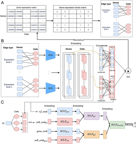
Overall workflow of the proposed GMFGRN approach. (A) Conversion of single-cell expression matrices to gene–cell heterogeneous graph. Specifically, we partitioned each expression value into its corresponding expression level and treated each expression level as an edge type in the heterogeneous graph. (B) Self-supervised training module that uses GCN to learn low-dimensional embeddings of genes and cells on the gene–cell heterogeneous graph by reconstructing gene expression data. (C) Supervised module that uses MLPs to identify TF–gene interactions based on gene embeddings and cell embeddings. |${MLP}_{classify}$| comprises three FC layers while the rest of the MLPs comprise two FC layers. There is a |$\mathrm{ReLU}$|activation function and Dropout applied between every two FC layers. The terms |$t{f}_{emb}$| and |$gen{e}_{emb}$| refer to the learned embeddings of the corresponding TF and gene in (B), respectively. |$cell\_ em{b}_{tf}$| (|$cell\_ em{b}_{gene}$|) denotes the average embeddings of all cells associated with the TF (gene), as learned in (B).
Construction of the gene–cell heterogeneous graph
We consider the single-cell expression matrix as a heterogeneous graph, where the non-zero values in the matrix are converted to 1 to generate the gene-to-cell adjacency matrix. In this heterogeneous graph, the edge’s properties represent the expression values of the corresponding genes in the cells. However, there exists a significant variation in gene expression across different cells, including extremely high or small gene expression values. This can pose challenges for the reconstruction of gene expression values. To deal with this, rather than applying self-supervised learning directly to the original heterogeneous graph, we instead divided each expression value into different scales, thereby obtaining various edge types in the heterogeneous graph. We then applied the self-supervised learning to this modified heterogeneous graph, as illustrated in Figure 1A and B.
Inspired by the 3DCEMA work [26], for a given gene expression matrix |$A$| (where rows represent genes and columns represent cells, respectively), we first obtained matrix |${A}^{\prime }$| by taking the logarithm of the non-zero values in the matrix to reduce the impact of the extreme expression values. We further discretized the expression values to remove the remaining extreme values. Specifically, for each gene |$i$| in |${A}^{\prime }$|, let |${A}_i^{\prime }=\left({a}_{i,1}^{\prime },{a}_{i,2}^{\prime },\dots, {a}_{i,c}^{\prime}\right)$| denote the expression vector of gene i including c cells. We calculated the mean |${u}_i$| and standard deviation |${std}_i$| of its non-zero values for |${A}_i^{\prime }$|. These were then used to determine the expression range of gene i across c cells, denoted as |${Value}_i$| as follows:
Next, we divided |$Valu{e}_i$| into |$n$| equidistant bins, where |$n$| is a hyperparameter that can be adjusted for different datasets. After this step, the range of the expression values of the |$k$|th bin of gene i can be calculated as follows:
Then, we assigned the corresponding bin index to the expression value of each gene in |${A}^{\prime }$| to obtain |${A}^{\prime \prime }$|. Specifically, for the |$i$|th gene, its expression value in the cell |$j$|can be redistributed as |${a}_{ij}^{\prime \prime }$|:
where k is referred to as the expression level of the gene |$i$| in the cell |$j$|. Considering each expression level as an edge type, the gene–cell heterogeneous graph constructed from matrix |${A}^{\prime \prime }$| would contain |$n$| edge types. As aforementioned, our proposed approach can learn the embeddings of both genes and cells on this heterogeneous graph.
Learning gene and cell embeddings with GCN
In the gene–cell heterogeneous graph, for each edge type, we set a GCN encoder for its individual processing. GCN consists of two main steps, i.e. message passing and aggregation. In the message passing step, the features of each node in the graph are nonlinearly transformed and passed on to the target node via the edges. For an edge type |$k$|, the message passing feature from the cell |$j$| to the gene |$i$| can be calculated as follows:
where |${c}_{ij}$| is a symmetric normalization constant, i.e. |$\sqrt{\left|{N}_i\right|\left|{N}_j\right|}$|, where |${N}_i$| denotes the set of neighbors of node |$i$| (note that the neighbors here include all edge types), |${W}_k$| is a specific edge type parameter matrix and |$cell\_{x}_j$| represents the initial random feature vector of cell |$j$|. Then, the features of gene |$i$| can be obtained at the message aggregation step as follows:
where |$gene\_{emb}_i$| represents the embedding of gene i, |$\parallel$| denotes the concatenation operation, |$n$| is the total number of edge types, i.e. the total number of expression levels, |${N}_{i,n}$| denotes all the neighbors of gene |$i$| with the edge type |$n$|, |$\sigma$| denotes the |$ReLU$| activation function and |${W}_{out}$| represents a trainable parameter matrix, respectively. Message passing from genes to cells was performed in a manner similar to aggregation. It is noteworthy that we used only one GCN layer for each edge type to prevent oversmoothing caused by deep layers [48]. To provide a more intuitive representation in the calculation process, we implement the above formula using matrix multiplication. Formulas (4) and (5) can be transformed into the following expressions:
where |${\overset{\sim }{A}}_k$| represents the adjacency matrix of edge type k, with dimensions |$g\times c$|, where g denotes the number of genes and c represents the number of cells. X denotes the random initialization features of gene and cell nodes, with a dimension of |$\left(g+c\right)\times em{b}_{size}$|, where |$em{b}_{size}$| is the dimensionality of the initialization features. D represents the diagonal node degree matrix with non-zero elements |${D}_{ii}=\left|{N}_i\right|$|. |${H}_k$| represents the output of the GCN for edge type k. |${H}_{genes}$| and |${H}_{cells}$| respectively represent the concatenation of features in the output of GCN corresponding to each edge type. |$Gen{e}_{embs}$| and |$Cel{l}_{embs}$| represent the final embeddings of all genes and cells outputted by the self-supervised model.
We performed the Z-score normalization on the original gene expression matrix |$A$| while disregarding the 0 values when calculating the mean and variance. For each non-zero expression value in matrix A, we fit its normalized values using the inner product of the corresponding gene and cell embeddings and minimized the MSE loss with the following equation:
where |$M$| denotes the count of non-zero expression values in matrix A,|$gene\_{emb}_m$| and |$cell\_{emb}_m$| denote the gene embedding and cell embedding associated with the |$m$|th expression value, respectively, ‘·’ denotes the dot product, while |$scor{e}_m$| represents the |$m$|th expression value, respectively.
Using MLP to identify gene interactions
At the previous stage, we applied self-supervised learning to learn the low-dimensional embeddings of each gene and cell. At the current stage, we then used the learned gene embeddings to infer gene interactions: First, for a TF–gene pair |$\left( tf, gene\right)$|, we obtained embeddings for |$tf$| and |$gene$|, denoted as |$tf\_ emb$| and |$gene\_ emb$|, respectively. Second, the embeddings of the cells associated with |$tf$| (|$gene$|) were averaged to generate |$cell\_{emb}_{tf}$| (|$cell\_{emb}_{gene}$|). Finally, these four embeddings were fed into the network model, as shown in Figure 1C for model training. Specifically, we first used two multi-layer perceptrons (MLPs) to extract the features of gene embedding and cell embedding, respectively, using the following equations:
where both |$ML{P}_{gene}$| and |$ML{P}_{cell}$| consist of two FC layers, with a |$ReLU$| activation function and Dropout applied after the first layer. Dropout was used to prevent overfitting of the model. Next, |$tf\_{emb}^{\prime }$| (|$gene\_{emb}^{\prime }$|) was concatenated with |$cell\_{emb}_{tf}^{\prime }$| (|$cell\_{emb}_{gene}^{\prime }$|) and fed into |$ML{P}_{gc1}$| (|$ML{P}_{gc2}$|) to extract the deep features of the gene and its corresponding cell. Finally, the outputs of these two MLPs were further concatenated together and fed into the final MLP layer for making the classification using the following equation:
where |$ML{P}_{gc1}$| and |$ML{P}_{gc2}$| consist of two FC layers each, while |$ML{P}_{classify}$| consists of three FC layers. Note that there is a |$ReLU$| activation function and Dropout applied between every two FC layers.
Benchmarking datasets
In this study, we employed eight static scRNA-seq datasets and four time-series scRNA-seq datasets to comprehensively evaluate and validate the performance of our proposed GMFGRN approach. In the static datasets, three cell lines did not contain pseudotime, including dendritic cells [49], bone marrow-derived macrophages [49] and IB10 mouse embryonic stem cells (mESC(1)) [50]. However, the pseudotime information was included in the other five cell lines, including two embryonic stem cell (hESC) datasets [51], the 5G6GR mouse embryonic stem cell (mESC(2)) dataset [52] and three mouse hematopoietic stem cell line datasets [53] (erythroid lineage (mHSC(E)), granulocyte-macrophage lineage (mHSC(GM)) and lymphoid lineage (mHSC(L))). We preprocessed and normalized these eight scRNA-seq datasets according to the procedures described in [3, 6]. For each dataset, the corresponding ground truth network was obtained from the ChIP-seq data [3, 6].
To examine the prediction performance of GMFGRN, we further collected four time-series scRNA-seq datasets, including two human embryonic stem cell datasets (hESC1 and hESC2) [51, 54] and two mouse datasets (mESC1 and mESC2) [50, 55], from the Gene Expression Omnibus [56] and ArrayExpress databases [57]. We selected 36 TFs for hESC1, hESC2 and mESC1 and 38 TFs for mESC2, respectively. The corresponding ground truth networks were again obtained from the ChIP-seq data available in the Gene Transcription Regulation Database [58]. In addition, for each positive TF–gene pair in each dataset, we randomly selected genes for the TF that did not interact with it, thereby ensuring that each TF had the same number of positive genes as negative genes. A statistical summary of each data set is provided in Tables 1 and 2. In the subsequent experiments, we fixed the embedding size of the genes and cells learned by GMFGRN to 256 and the number of expression levels to 15 or 25 depending on the dataset. Detailed analyses of the impact of these two hyperparameters on the model performance are discussed in the ‘Ablation experiments’ section. The settings for the other hyperparameters are provided in Supplementary Text S4, which also includes detailed computational information about the implementation of GMFGRN, including the programming language used and the framework employed.
Statistical summary of the eight static scRNA-seq datasets used in this study
| Cell line | Number of genes | Number of cells | Size of training set | Number of TFs | Pseudotime |
|---|---|---|---|---|---|
| Bone marrow-derived macrophages | 20 463 | 6283 | 50 254 | 13 | N |
| Dendritic cells | 20 463 | 4126 | 28 046 | 16 | N |
| mESC(1) | 24 175 | 2717 | 154 931 | 38 | N |
| hESC | 17 735 | 758 | 77 151 | 18 | Y |
| mESC(2) | 18 385 | 421 | 150 541 | 18 | Y |
| mHSC(E) | 4762 | 1071 | 44 735 | 18 | Y |
| mHSC(GM) | 4762 | 889 | 44 741 | 18 | Y |
| mHSC(L) | 4762 | 847 | 44 738 | 18 | Y |
Statistical summary of the four time-course scRNA-seq datasets used in this study
| Datasets | Number of genes | Number of cells | Time points | Accession number |
|---|---|---|---|---|
| mESC1 | 19 427 | 3456 | 9 | GSE79758 |
| mESC2 | 24 175 | 2717 | 4 | GSE65525 |
| hESC1 | 26 178 | 1529 | 5 | E-MTAB-3929 |
| hESC2 | 19 189 | 758 | 6 | GSE75748 |
| Datasets | Number of genes | Number of cells | Time points | Accession number |
|---|---|---|---|---|
| mESC1 | 19 427 | 3456 | 9 | GSE79758 |
| mESC2 | 24 175 | 2717 | 4 | GSE65525 |
| hESC1 | 26 178 | 1529 | 5 | E-MTAB-3929 |
| hESC2 | 19 189 | 758 | 6 | GSE75748 |
Performance benchmarking of different methods
Using the eight static datasets, we benchmarked GMFGRN with 12 widely used unsupervised and supervised approaches. The unsupervised methods included PCC, MI, PIDC [13], GENIE3 [19], SCODE [16], SINCERITIES [17], Normi [22], NG-SEM [21] and MetaSEM [23]. Supervised methods include CNNC [3], DeepDRIM [4] and STGRNS [29]. Using the four time-series datasets, we also compared the performance of GMFGRN with that of three unsupervised methods (PCC, MI and dynGENIE3 [35]) and four supervised methods (TDL-3DCNN [27], TDL-LSTM [27], dynDeepDRIM [5] and STGRNS [29]). A detailed description of the parameter settings for these compared methods is provided in Supplementary Texts S1 and S2. To compare supervised approaches, 3-fold cross-validation was used to evaluate the model and ensure that there were no overlapping TFs between the training and testing sets. We retrained the models of the benchmarked methods and ensured that all methods used the same partitioning ratios of the datasets for training and testing, respectively.
RESULTS
Performance comparison of GMFGRN and existing methods on eight static datasets
In this section, we benchmarked the performance of GMFGRN with PCC, MI, Normi, MetaSEM, CNNC, DeepDRIM and STGRNS on eight static scRNA-seq datasets (Table 1). Among these methods, PCC, MI, Normi and MetaSEM are unsupervised methods while CNNC, DeepDRIM and STGRNS are state-of-the-art supervised learning-based approaches. Figure 2A–D demonstrates that supervised methods generally outperformed unsupervised methods. GMFGRN outperformed DeepDRIM on all datasets, with improvements in terms of AUROC. Specifically, the AUROC of GMFGRN increased 1.28, 1.96, 2.43 and 6.04% compared to that of DeepDRIM on the bone marrow-derived macrophage, dendritic cell, hESC and mESC(1) datasets, respectively. The heatmaps of AUROC and AUPRC for all compared methods on the eight datasets are shown in Figure 2C and D. As can be seen, GMFGRN achieved an average AUROC of 0.797 and an average AUPRC of 0.760 on the eight datasets, both of which were higher than those of the second-best method DeepdRIM (i.e. with an average AUROC and AUPRC of 0.778 and 0.735, respectively). In terms of the ACC and MCC metrics, the results can be found in Supplementary Tables S1 and S2, from which we can see that GMFGRN outperformed DeepDRIM on five and six static datasets, respectively. GMFGRN achieved a maximum increase of 4.3% in terms of ACC and 9.1% in terms of MCC, respectively. We calculated the AUROC and AUPRC values for each TF on the eight static datasets by the eight methods (Supplementary Tables S6 and S7). We also performed the Wilcoxon signed-rank test to calculate the P-values between GMFGRN and DeepDRIM in terms of AUROC and AUPRC of TFs on eight static datasets. The detailed results are provided in Supplementary Table S5. According to the P-values, GMFGRN achieved a performance similar to that of DeepDRIM on most datasets. However, it is noteworthy that the training time and memory consumption of GMFGRN were significantly lower than those of DeepDRIM. These aspects will be elaborated on in the subsequent sections. In addition, we computed the numbers of false-positive samples of GMFGRN on the eight datasets. As shown in Figure 2E, GMFGRN efficiently eliminated false positives resulting from transitive interactions, even without considering the neighbor information. This is presumably due to the principle that GNN uses to aggregate the neighbor information to update the node’s information. By utilizing cell nodes as bridges, the genes with the same cell can share information with each other and can thereby eliminate transitive interactions [4]. However, as can be seen from Figure 2E, although STGRNS had the lowest number of false positives, it also generated a notably high number of false negatives, as shown in Supplementary Figure S1. Therefore, taking into consideration other metrics, its performance was not as outstanding as that of GMFGRN.
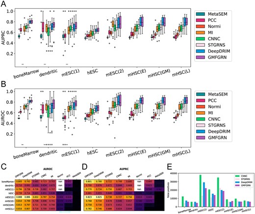
Comparison of GMFGRN with existing state-of-the-art approaches for predicting TF–gene interactions on eight static datasets. (A, B) Box plots and (C, D) heatmaps of AUROC and AUPRC of GMFGRN and compared methods on eight static datasets. The symbol ‘nan’ indicates that it took the Normi method too long to run on these datasets, and its results could not be obtained. (E) Comparison of the numbers of false positives predicted by GMFGRN, DeepDRIM, STGRNS and CNNC on eight static datasets.
In addition, we further compared GMFGRN with the four most advanced unsupervised methods reported in BEELINE [6], including PIDC [13], GENIE3 [19], SCODE [16] and SINCERITIES [17]. Another recent unsupervised method, NG-SEM [21], has been also included in the performance comparison. Considering that some approaches require pseudotime information, we chose five datasets with pseudotime for comparison, including hESC, mESC(2), mHSC(E), mHSC(GM) and mHSC(L). To improve the performance of the unsupervised methods, we selected the top-varying 500 genes for each dataset. All the methods were validated on the TFs/genes in the cross-validation test dataset that overlap with the top-varying 500 genes. The results in Figure 3 show that GMFGRN outperformed DeepDRIM on four of the five datasets, including hESC, mHSC(E), mHSC(GM) and mHSC(L), with an average AUROC increase of 1.13% over DeepDRIM. Taken together, these results show that GMFGRN performed better than DeepDRIM and other unsupervised methods.
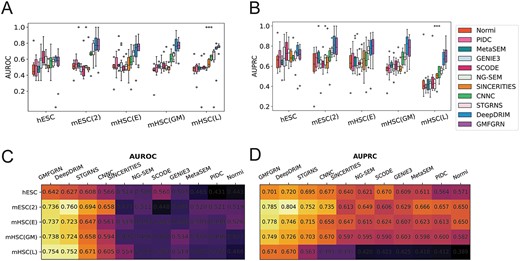
Comparison of GMFGRN with other existing approaches on the top-varying 500 gene pairs across five datasets. AUROC and AUPRC values are presented using (A, B) boxplots and (C, D) heatmaps.
Performance comparison of GMFGRN and other methods on four time-series datasets
It is noteworthy that we did not develop an ad hoc module for handling time-series data in GMFGRN, but instead, we combined the gene expression data from various time points and utilized the merged gene expression data to conduct self-supervised training and then supervised training. We compared the performance of GMFGRN and seven state-of-the-art methods specifically designed for time-series scRNA-seq data, including three unsupervised methods (dynGENIE3 [35], PCC and MI) and four supervised methods (TDL-3DCNN [27], TDL-LSTM [27], dynDeepDRIM [5] and STGRNS [29]). dynGENIE3 was designed for bulk RNA-seq data while other methods were implemented for processing scRNA-seq data. For time-series data, we averaged the gene expression values of all cells at each time point and used these values as input to dynGENIE3. The performance comparison results are shown in Figure 4. As can be seen, the AUROC values of GMFGRN on mESC2, hESC1 and hESC2 were higher than those of the second-best method dynDeepDRIM, with a maximum increase of 2.4 and 1.3% in terms of AUROC and AUPRC, respectively. The performance results in terms of the ACC and MCC metrics can also be found in Supplementary Tables S3 and S4. The results indicate that GMFGRN outperformed dynDeepDRIM in terms of ACC and MCC on both the hESC1 and hESC2 datasets. As shown in the boxplots, the AUROC of GMFGRN was more stable and less variable than the other approaches. Its performance improvement might be attributed to the fact that the other supervised methods need to change the model structure when dealing with the data with different time points, while GMFGRN combines the gene expression matrices of all time points and unify them for model training, and as such, it can avoid this situation and facilitate the migration between different datasets. In addition, specific AUROC values and AUPRC values are provided for each TF on the four time-series datasets by the eight methods, which can be found in Supplementary Tables S8 and S9. The P-values for the AUROC and AUPRC metrics of GMFGRN and dynDeepDRIM can be found in Supplementary Table S5. The results suggest that the performance of GMFGRN is comparable to dynDeepDRIM.
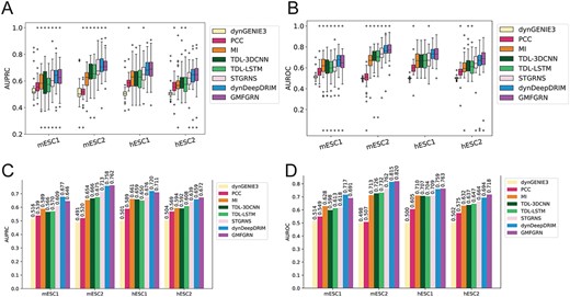
Performance comparison of GMFGRN with seven other existing methods on four time-series datasets. (A, B) Boxplots and (C, D) bar charts of AUPRC and AUROC for the eight methods across four time-series scRNA-seq data.
Evaluation of computational complexity and memory consumption
Apart from the conventional performance measures, training time and memory consumption are the other two important criteria to assess the feasibility of model training. Accordingly, we selected the second-best DeepDRIM on static scRNA-seq datasets and dynDeepDRIM on time-series datasets to benchmark the training time and consumed memory with our GMFGRN. We selected all the time-series datasets and three static datasets with the largest numbers of training samples, i.e. mESC(1), mESC(2) and hESC. All methods were run on NVIDIA GeForce RTX 3090. According to Table 3, GMFGRN’s training time (including both self-supervised and supervised training) was generally 10% less than the training time required by DeepDRIM and dynDeepDRIM on all six large datasets. For example, the training time of GMFGRN on the mESC(2) and mESC1 datasets was only 4.55 and 2.52% of the training time of the compared methods, respectively. Furthermore, GMFGRN exhibited minimal memory requirements. For instance, on the mESC(2) dataset, the memory required by GMFGRN is only 8.55% of the memory consumption by DeepDRIM. These results indicate that GMFGRN can predict TF–gene interactions both accurately and efficiently with less required time and memory. Note that the term ‘memory’ here refers to the main memory, instead of the GPU memory, because the GPU memory can be influenced by various factors such as the batch size and model parameter size, while the main memory is only affected by the size of the dataset. To fully validate the superiority of the gene embeddings learned by GMFGRN (in terms of less memory consumption), we used main memory consumption as the metric to make the comparison. In addition, in terms of GPU memory, the memory consumption of GMFGRN was also lower than that of the second-best method.
Comparison of training time and consumed memory of DeepDRIM, dynDeepDRIM and GMRGRN on seven large-scale scRNA-seq datasets
| Dataset | DeepDRIM | dynDeepDRIM | GMFGRN | |||
|---|---|---|---|---|---|---|
| Training (h) | Memory (GB) | Training (h) | Memory (GB) | Training (h) | Memory (GB) | |
| hESC | 8.00 | 34.06 | – | – | 0.78 | 3.80 |
| mESC(1) | 10.11 | 56.34 | – | – | 0.86 | 7.08 |
| mESC(2) | 11.64 | 53.24 | – | – | 0.53 | 4.55 |
| hESC1 | – | – | 22.14 | 27.09 | 0.84 | 5.90 |
| hESC2 | – | – | 14.98 | 27.64 | 0.65 | 4.71 |
| mESC1 | – | – | 29.72 | 33.81 | 0.75 | 4.77 |
| mESC2 | – | – | 22.29 | 22.39 | 0.87 | 7.08 |
Ablation experiments
Multiple factors may affect the performance of GMFGRN, including dropout events, number of time points in scRNA-seq data and parameter settings. To comprehensively evaluate the predictive performance of GMFGRN, we conducted a series of ablation experiments using the bone marrow-derived macrophage and hESC1 datasets (Figure 5). The bone marrow-derived macrophage was used to assess the performance differences of GMFGRN with varying embedding vector sizes, number of expression levels and number of edges in the gene–cell heterogeneous graph, while hESC1 was used to evaluate the performance differences of GMFGRN with different numbers of time points.
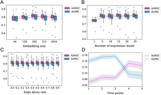
Ablation experiments to assess the impact of different parameters on the performance of GMFGRN on bone marrow-derived macrophages dataset and hESC1 dataset. (A–C) The impact of different embedding size, number of expression levels and number of gene–cell heterogeneous graph edges on the performance of GMFGRN based on bone marrow-derived macrophages. (D) The impact of different time points on the performance of GMFGRN on hESC1 dataset.
Effect of gene–cell embedding size
The size of the embedding vector refers to the dimensionality of gene and cell representations in the embedding space. In this section, we investigated the impact of different sizes of gene–cell embeddings on the performance of our model using different sizes, including 64, 128, 256, 512 and 1024. Figure 5A shows AUROC and AUPRC values of GMFGRN on the bone marrow-derived macrophages dataset with various embedding sizes. We observed that smaller embedding sizes (e.g. 64) resulted in lower model performance, presumably due to the limited capacity of smaller embedding vectors to capture the intricate relationships between genes and cells. As the embedding size gradually increased, there was an improvement in model performance. However, further increasing the embedding vector size might have introduced noise into the model, leading to reduced performance (e.g. dimension 1024). While excessively small or large dimensions may cause a slight decline in model performance, overall, the size of the embedding vector does not exert a significant influence on model performance. Based on the performance shown in Figure 5A, we chose the embedding size of 256 across all datasets.
Effect of the number of expression levels
During the self-supervised training phase, we divided the gene expression values into different expression levels and constructed a gene–cell heterogeneous graph containing multiple edge types. Here, we assessed the effect of the number of different expression levels on the model performance. In particular, we introduced a parameter |$n$| to represent the number of expression levels and accordingly modified the expression values to an integer between 1 and |$n$|. Figure 5B shows the AUROC and AUPRC values of the bone marrow-derived macrophages dataset with different numbers of expression levels |$n$|. As can be seen, the performance of the model was lower when the number of expression levels was set to 1 (i.e. only one edge type). This indicates that there were too many extreme values in gene expression values, and it would be difficult to fit all expression values with one GCN. However, when the number of expression levels exceeded 5, GMFGRN exhibited similar performance, indicating that our model is robust to different numbers of expression classes. Therefore, in our experiments, the number of expression levels was set to 15 or 25 for all datasets depending on the performance. A detailed description of this parameter setting can be found in the ‘ReadMe’ file in our GitHub repository available at https://github.com/Lishuoyy/GMFGRN.
Effect of the number of edges in the heterogeneous graph
We further examined the effect of the number of edges in the gene–cell heterogeneous graph on the model performance. Specifically, we randomly removed 10% to 90% of the number of edges in the gene–cell heterogeneous graph on the bone marrow-derived macrophages dataset. The higher number of deleted edges also indicates an increase in the dropout rate of the gene expression matrix. To ensure a fair comparison, we repeated the experiments 10 times and reported the average performance results (Figure 5C). GMFGRN showed stable performance with respect to different numbers of edges, and achieved a better performance even if only 10% of edges were retained. The results suggest that GMFGRN is robust to the change of the dropout rate.
Effect of the number of time points
In contrast to static datasets, time-series datasets often include multiple time points. Therefore, we further investigated the performance of GMFGRN with respect to different numbers of time points on the hESC1 dataset. We divided the hESC1 dataset into five sub-datasets, with each sub-dataset set with a different number of time points, including {t1}, {t1, t2}, …, {t1, t2, t3, t4, t5}. Figure 5D displays the median AUROC and AUPRC of GMFGRN at different time points where the shaded area represents the standard error. As shown in Figure 5D, the AUROC value of GMFGRN increased gradually with the increase of time points while the AUPRC value dropped starting from the third time point. Although AUPRC started to decline from the third time point, this metric focuses on the accuracy of positive class samples, while AUROC emphasizes on the model’s classification ability, especially the trade-off between the true-positive rate and false-positive rate at different probability thresholds. In the context of this study, our primary focus lies in evaluating the overall classification capability of the model, with particular attention to enhancing the AUROC metric. As evident from Figure 5D, an increase in the number of involved time points correlates positively with higher AUROC values. Therefore, we conclude that the temporal information of time-series scRNA-seq data is of critical importance, and the data from all time points should be fully considered during model training to obtain more accurate and comprehensive results.
Showcasing the prediction power of GMFGRN
In this section, we conducted a case study to further assess the predictive capability of GMFGRN to identify potential target genes for a specific TF. We conducted this experiment on the hESC2 dataset. We first used the entire training set to train GMFGRN and applied the trained model to predict the entire GRNs on the hESC2 dataset. Specifically, we used the trained GMFGRN to predict unknown TF–gene pairs of TFs in hESC2. The network containing the top-100 predicted TF–gene interactions is displayed in Figure 6C. In addition, we focused on predicting the target genes of transcription factors TAF1 (TATA-box binding protein associated factor 1) and TBP (TATA-binding protein). Figure 6A and B shows the top 20 potential target genes sorted by predicted scores for TAF1 and TBP, respectively. Both TAF1 and TBP participate in the formation of the transcription initiation complex. TAF1 also interacts with activators and other transcriptional regulatory factors, and these interactions influence the rate of transcription initiation [59]. Mutations in the TAF1 gene result in Dystonia 3, torsion, X-linked, a form of Dystonia-Parkinsonism syndrome [60]. TBP is a key member of the transcription initiation factor complex, and its abnormal expression or mutations are associated with diseases such as cancer, neurodegenerative disorders and immunodeficiency [61]. We manually validated the top 20 predicted target genes of TAF1 and TBP in the Harmonizome database [62]. Among the top 20 predicted target genes of TAF1, 15 have been experimentally validated, while all the top 20 predicted target genes of TBP have been experimentally validated. A detailed list of these validated genes is provided in Supplementary Table S10. These results illustrate the effectiveness of GMFGRN in predicting novel potential target genes of transcription factors.
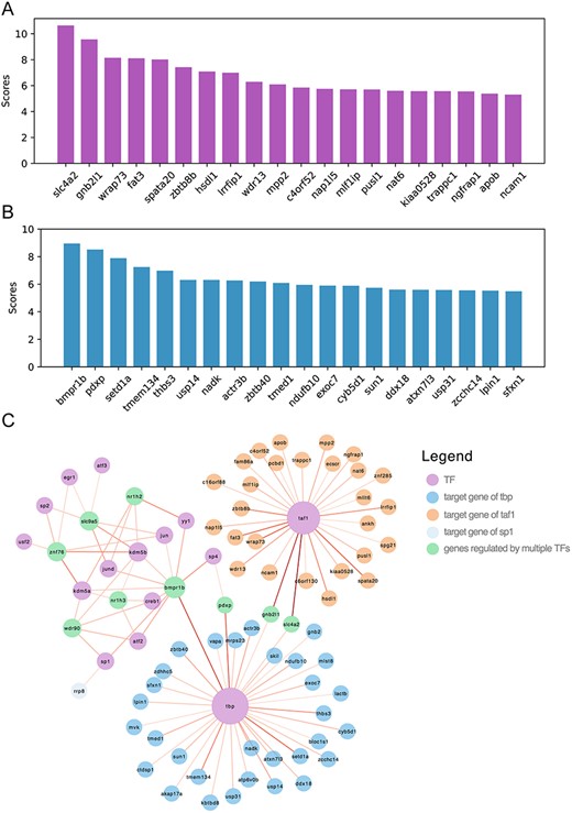
Application of GMFGRN to predict potential target genes in the hESC2 dataset. (A, B) Ranking plots of the top 20 predicted potential target gene scores for TAF1 and TBP. (C) Visualization of the gene regulatory networks predicted by GMFGRN. The size of the node is positively correlated with the degree. The depth of edge shadow was positively correlated with the predicted scores.
CONCLUSION
In this study, we have developed a new deep-learning-based approach, termed GMFGRN, for inferring GRNs from scRNA-seq data. GMFGRN makes no assumptions about or imposes any constraints on the scRNA-seq data, thereby representing it as a flexible and adaptive approach with an excellent potential for further applications across diverse scenarios. The attractive feature of GMFGRN involves the factorization of the single-cell expression matrix using Graph Convolutional Neural Networks (GCN). This enables effective learning of the embeddings for both genes and cells through the reconstruction of gene expression values. Subsequently, the learned embeddings of TF–gene pairs and their associated cell embeddings are fed into an MLP classifier to predict the interactions between TFs and genes. Importantly, GMFGRN leverages the message passing and aggregation processes of GCN, which effectively alleviate the indirect regulation issue induced by transitive interactions and thereby reduce the false-positive rate. The large sparsity of the single-cell expression matrix and low complexity of MLP allow GMFGRN to reduce the training time. Benchmarking experiments on eight static datasets and four time-series scRNA-seq datasets demonstrate that GMFGRN not only outperformed state-of-the-art approaches but also reduced training time and memory consumption. In addition, the learning strategy utilized by GMFGRN can be broadly applied to various bioinformatics tasks associated with scRNA-seq data, such as cell clustering and type identification using the learned cell embeddings. We anticipate that GMFGRN can serve as a fast and accurate tool for reliable inference of GRNs from scRNA-seq data.
Despite the promising performance of GMFGRN, several issues still exist. First, as the self-supervised training in GMFGRN relies on GCN, the cold start problem needs to be addressed. Particularly, when a new gene node is added, GMFGRN can only be retrained to predict its interactions with other genes. Second, we did not design an ad hoc method to predict the regulatory direction, but only the regulatory interaction. Third, for the time-series datasets, we did not leverage the full temporal dimension information but only concatenated the data from all time points. In future work, we plan to design self-supervised and downstream modules of GMFGRN to solve the above issues and explore strategies to improve the performance of GMFGRN in inferring gene regulatory networks from time-series data.
We propose a two-stage deep-learning-based approach, termed GMFGRN, to infer gene regulatory networks from scRNA-seq data.
GMFGRN is capable of learning representative gene and cell embeddings from heterogeneous gene–cell graphs via graph convolutional networks (GCNs), thereby effectively eliminating false positives due to transitive interactions.
We illustrate the advanced performance of GMFGRN on 12 scRNA-seq data sets, as well as its lower requirement for computational resources including memory consumption and training time compared to other supervised methods for gene regulatory network inference.
We also showcase the predictive power of GMFGRN in effectively identifying potential target genes for specific transcription factors.
FUNDING
The National Natural Science Foundation of China (62372234, 62072243, 61772273); Natural Science Foundation of Jiangsu (No. BK20201304); Foundation of National Defense Key Laboratory of Science and Technology (JZX7Y202001SY000901); Major and Seed Inter-Disciplinary Research (IDR) projects awarded by Monash University.
DATA AVAILABILITY
The datasets used in this paper are downloaded from https://zenodo.org/record/8418696.
Author Biographies
Shuo Li received his BEng degree in computer science from Yancheng Institute of Technology in 2021. He is currently a master’s candidate in the School of Computer Science and Engineering, Nanjing University of Science and Technology, and a member of the Pattern Recognition and Bioinformatics Group. His research interests include pattern recognition, machine learning and bioinformatics.
Yan Liu received his PhD degree in computer science from Nanjing University of Science and Technology in 2023. He is currently a young hundred distinguished professor with the School of Information Engineering, Yangzhou University, China. His research interests include pattern recognition, machine learning and bioinformatics.
Long-Chen Shen received his MS degree in software engineering from Nanjing University of Science and Technology in 2021. He is a PhD candidate in the School of Computer Science and Engineering, Nanjing University of Science and Technology, and a member of the Pattern Recognition and Bioinformatics Group. His current interests include pattern recognition, data mining and bioinformatics.
He Yan received his MS degree from Nanjing Forestry University, China, in 2014, and PhD degree from Nanjing University of Science and Technology, China, in 2017. He is currently a postdoc in the School of Computer Science and Engineering, Nanjing University of Science and Technology. From 2019 to 2021, he acted as a visiting scholar at the University of Alberta in Canada. His research interests include machine learning, intelligent transportation systems, data mining and its applications.
Jiangning Song is an associate professor and group leader in the Monash Biomedicine Discovery Institute and the Department of Biochemistry and Molecular Biology, Monash University, Melbourne, Australia. He is also a member of the Monash Data Futures Institute and Alliance for Digital Health at Monash University. His research interests include bioinformatics, computational biomedicine, machine learning, data mining and pattern recognition.
Dong-Jun Yu received his PhD degree from Nanjing University of Science and Technology in 2003. He is currently a full professor in the School of Computer Science and Engineering, Nanjing University of Science and Technology. His research interests include pattern recognition, machine learning and bioinformatics. He is a senior member of the China Computer Federation (CCF) and a senior member of the China Association of Artificial Intelligence (CA).
References
Author notes
Shuo Li and Yan Liu contributed equally to this work.
