


Abstract
Numerous biological studies have shown that considering disease-associated micro RNAs (miRNAs) as potential biomarkers or therapeutic targets offers new avenues for the diagnosis of complex diseases. Computational methods have gradually been introduced to reveal disease-related miRNAs. Considering that previous models have not fused sufficiently diverse similarities, that their inappropriate fusion methods may lead to poor quality of the comprehensive similarity network and that their results are often limited by insufficiently known associations, we propose a computational model called Generative Adversarial Matrix Completion Network based on Multi-source Data Fusion (GAMCNMDF) for miRNA–disease association prediction. We create a diverse network connecting miRNAs and diseases, which is then represented using a matrix. The main task of GAMCNMDF is to complete the matrix and obtain the predicted results. The main innovations of GAMCNMDF are reflected in two aspects: GAMCNMDF integrates diverse data sources and employs a nonlinear fusion approach to update the similarity networks of miRNAs and diseases. Also, some additional information is provided to GAMCNMDF in the form of a ‘hint’ so that GAMCNMDF can work successfully even when complete data are not available. Compared with other methods, the outcomes of 10-fold cross-validation on two distinct databases validate the superior performance of GAMCNMDF with statistically significant results. It is worth mentioning that we apply GAMCNMDF in the identification of underlying small molecule-related miRNAs, yielding outstanding performance results in this specific domain. In addition, two case studies about two important neoplasms show that GAMCNMDF is a promising prediction method.
INTRODUCTION
Micro RNAs (miRNAs) are endogenous noncoding RNAs with regulatory functions whose mutation or abnormal expression is related to diverse biological processes [1]. In light of the progress made in human genetic engineering, the important biological functions of miRNAs have also been linked to the diagnosis and therapeutic approaches for human diseases [2]. Accurate prediction of miRNA–disease associations (MDAs) can contribute to unraveling disease mechanisms and identifying novel drug candidates [3].
However, there are some limitations to using experimental means to uncover novel interactions between diseases and miRNAs, such as being small-scale and time-consuming. The exponential growth of biological data and the rapid advancement of intelligent technologies have led to the emergence of numerous viable computational models. These models offer cost-effective alternatives to guide biological experiments.
Under the premise that functionally related miRNAs are inclined to be involved in diseases exhibiting similar phenotypes, Guo et al. [4] introduced a model using a multilayer linear projection (MLPMDA), which introduced multiple layers of linear projections to capture the interaction information. The shortcoming of this model was that it required a reliable data source for better performance. In their study, Zhang et al. [5] proposed a weighted tuning approach (WVMDA), which incorporated a similarity filtering method. Niu et al. [6] proposed a binary logistic regression method (RWBRMDA) that utilized the random displacement of feature vectors extracted from each miRNA. By leveraging these feature vectors along with marker information, RWBRMDA predicted the corresponding disease for the given miRNAs of interest. An original joint embedding model was presented by Liu et al. [7]. They used a gradient-boosting decision tree to extract highly insightful features from various data sources. Furthermore, numerous network-based models have been created. For instance, Peng et al. [8] established a two-layer network by extracting data from multiple sources. In another study, Zheng et al. [9] introduced a graph embedding approach that learned the probability distribution of miRNA–disease pairs within the biological network. They devised an effective computational model called iMDABN, which harnessed the power of network information to unveil unknown MDAs and demonstrated promising performance. Despite the advancements achieved by these methods in miRNA–disease prediction, it should be noted that some of them solely relied on miRNA functional similarity, potentially introducing bias toward functional aspects of miRNAs.
Over the past few years, deep learning methods, including convolutional neural networks, autoencoders and graph convolutional networks, have gained widespread adoption in the study of MDAs. Ding et al. [10] used a deep learning framework VGAE-MD. It should be noted that the framework involved the utilization of two deep learning networks, contributing to a higher level of algorithmic complexity. Li et al. [11] combined miRNA and disease embeddings and utilized graph convolutional autoencoder to capture their complex relationships within the biological network. Although it could effectively capture the network information and achieve high prediction accuracy, there were problems in processing high-dimensional data. Li et al. [12] employed a novel approach to effectively complete the neural induction matrix for identifying MDAs. Nevertheless, its downsides maybe its high computational complexity and the need for large amounts of data. The above methods used the average of the different types of similarities to obtain a comprehensive similarity network. However, they may be subject to coverage errors, scale errors and noise of the different similarities, which may result in poor quality of the integrated similarity network. Consequently, the incorporation of diverse data sources can potentially impact the precision of the model.
Specifically, the utilization of matrix completion techniques has proven to be a valuable approach in the prediction of MDAs. Xuan et al. [13] specifically focused on the deep integration of miRNA family and cluster features and used a nonnegative matrix with sparsity constraints for prediction. However, they did not perform well because they only considered local network similarity. Li et al. [14] used both linear and nonlinear similarity measures, which could effectively handle missing data and achieve high prediction accuracy. However, the drawback might be that nonlinear relationships can only be captured to a limited extent. Building upon MCMDA, Chen et al. [15] made enhancements and introduced IMCMDA, a refined model that demonstrated superior performance. Chen et al. [16] created NCMCMDA, which could effectively handle missing data and achieve high prediction accuracy. However, the drawback could be its high computational complexity.
Despite the remarkable achievements of previous matrix completion-based approaches, it is important to note that many of them heavily relied on available association data, making them susceptible to the influence of noisy information. Moreover, some methods cannot restrict the prediction results to [0,1]. To solve the above problems, inspired by the Generative Adverse Networks method [17], we propose an effective method: GAMCNMDF. The flowchart for GAMCNMDF is displayed in Figure 1. Initially, we incorporated miRNA sequence similarity as an additional factor to enhance the accuracy of the integrated miRNA–miRNA similarity. Subsequently, utilizing a nonlinear fusion technique, GAMCNMDF constructed two extensive similarity networks for miRNA and disease by integrating diverse data sources. This approach proficiently captured both shared and distinctive information from multiple sources, demonstrating resilience to noise and heterogeneity in the data. After that, MDAs were then introduced to the heterogeneous network and served as a representation of it. The predictions made by GAMCNMDF were constrained to a range of [0, 1], ensuring the validity and interpretability of the results. To enhance the learning process of the discriminator and ensure it captured the desired distribution, an additional hint vector was introduced. This hint provided the discriminator with information about the missing components in the matrix, enabling it to focus its attention on specific components’ quality. By incorporating this hint, GAMCNMDF ensured that the generator learned to follow the true distribution of the data. Moreover, GAMCNMDF demonstrated favorable performance in inferring interactions between small molecule–miRNAs associations. To evaluate the prediction accuracy, 10-fold cross-validation was performed using two distinct datasets. In addition, case studies of predicted miRNAs were performed to confirm GAMCNMDF’s capacity to forecast potentially pertinent miRNAs for particular diseases. These outcomes are sufficient proof that the method works.
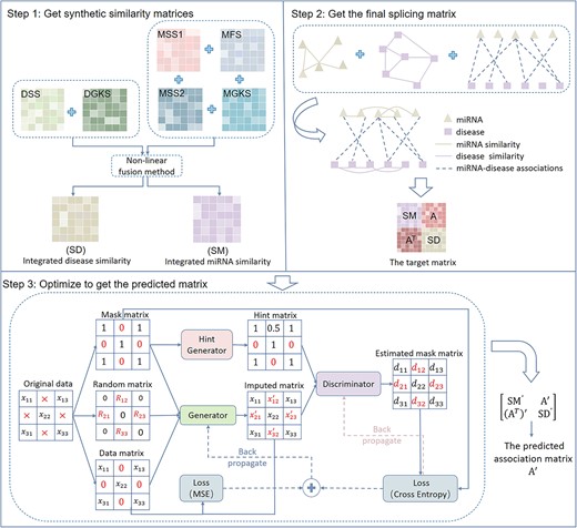
The flowchart of GAMCNMDF. (1) Get synthetic similarity matrices. (2) Get the final splicing matrix. (3) Optimize to get the predicted matrix, where gradient descent with momentum is used to optimize the aforementioned crucial equation.
MATERIALS AND METHODS
Datasets
Human MDAs
We employed two distinct datasets: HMDD v2.0 [18] and the corresponding datasets were acquired from a prior investigation [19]. Although both versions of the database contain some common information, they also have different features that are useful for MDAs. HMDD v3.2 is the newer version that contains more recent information. HMDD v2.0, on the other hand, although an older version, has a relatively large amount of data and contains more information about historically known MDAs. To ensure data consistency across various sources, a comprehensive approach was employed. This involved tagging HMDD v2.0 disease and miRNA names with miRBase, mirTarBase and MeSH descriptors. The resulting dataset included 6088 associations of 328 diseases and 550 miRNAs. Additionally, diseases and miRNAs that were present in HMDD v3.2 but not in MeSH and miRBase or mirTarBase were excluded. To create the association matrix, we finally obtained 8968 associations involving 788 miRNAs and 374 diseases. |$A \in R^{nm \times nd}$| is the MDA matrix, and |$nm$| and |$nd$| represented the total number of miRNAs and diseases, respectively. Table 1 displays the datasets.
Complete information about the datasets
| dataset | miRNAs | diseases | associations |
|---|---|---|---|
| HMDD v2.0 | 550 | 328 | 6088 |
| HMDD v3.2 | 788 | 375 | 8968 |
| dataset | miRNAs | diseases | associations |
|---|---|---|---|
| HMDD v2.0 | 550 | 328 | 6088 |
| HMDD v3.2 | 788 | 375 | 8968 |
Similarity networks
To provide more information for the prediction, different measures of similarity calculation are introduced based on different data sources. As shown in Figure 1, step 1, MSS1 denotes miRNA sequence similarity, MSS2 denotes miRNA semantic similarity, MFS denotes miRNA functional similarity, MGKS denotes miRNA GIP kernel similarity, DSS denotes diseases semantic similarity, DGKS denotes disease GIP kernel similarity, SD denotes disease comprehensive similarity, SM denotes miRNA comprehensive similarity, A denotes MDA matrix and |$\text{A}^{\text{T}}$| denotes the transpose of A.
MiRNA similarity networks. We calculated the following different types of miRNA similarity:
MiRNA sequence similarity. The sequence comparison algorithm is employed to calculate the miRNA sequence similarity, restricting the similarity value to [0,1] from a previous study [10]. Specifically, the miRNA sequences, comprising approximately 22 nucleotides ‘AUCG’, were acquired from the miRBase database. To determine the similarity value, we employed the ‘pairwise alignment’ functionality provided by the Biostrings R package. It is a function in R language to calculate the global or local pairwise score of two sequences. This function can be used to obtain the pairwise alignment score and sequence similarity between two sequences. For the calculation of sequence similarity, we utilized the ‘pairwise alignment’ function, applying specific parameters: a gap opening penalty of 5, a gap extension penalty of 2, a match score of 1 and a mismatch score of 1. The resulting miRNA sequence similarity matrix is denoted as |${SM}_{1}$|, with the similarity scores bounded within the range of [0,1].
MiRNA Gaussian interaction profile (GIP) kernel similarity. We calculated it using A in line with a previous method [20] to further analyze similarity. We denote it as |${SM}_{2}$|.
MiRNA semantic similarity. We utilized the gene ontology SemSim approach, which was previously introduced in [21], to obtain the resulting matrix, representing the semantic miRNA similarity, which is denoted as |${SM}_{3}$|.
MiRNA functional similarity. We determined the functional similarity and represented it as |${SM}_{4}$|, using a methodology similar to that of the preceding method [20].
Disease similarity networks. Two disease similarity networks were used:
Diseases Semantic similarity. We employed a previous study [22] which considered the shared portion in the directed acyclic graph and assumes that diseases with a larger shared portion exhibit higher semantic similarity. The final matrix is denoted as |${SD}_{1}$|.
Disease GIP kernel similarity. We calculated it using a similar approach as |${SM}_{2}$|’s calculation. Denote it as |${SD}_{2}$|.
Specifically, we performed miRNA and disease GIP kernel similarity matrices visualization in Figure 2. In each heat map, each row and column represents an miRNA or disease and each cell in the matrix represents the similarity between a pair of miRNAs or diseases, with values usually ranging from 0 to 1. The lighter the color, the higher the similarity between the two miRNAs or diseases.
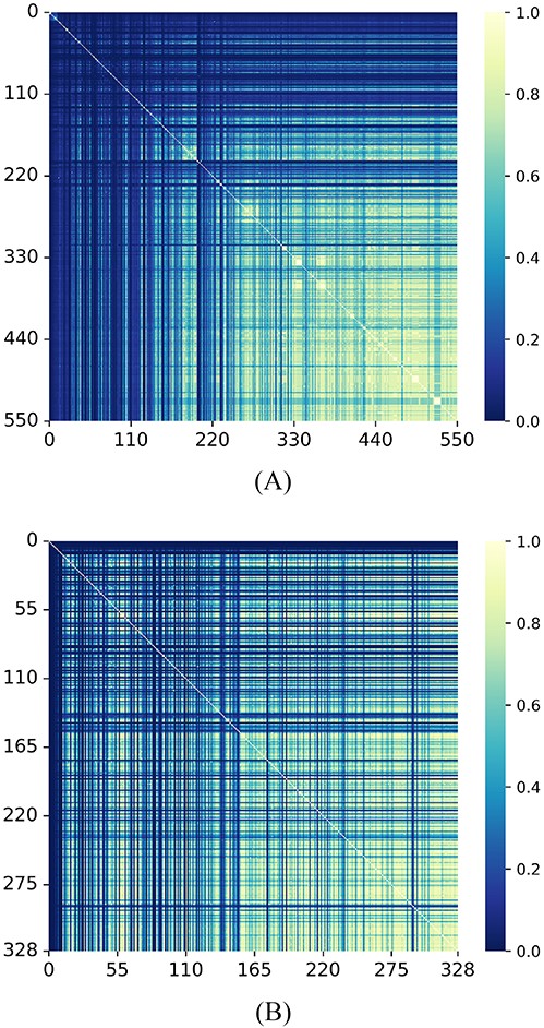
(A) Visualization of |${SM}_{2}$|(B) Visualization of |${SD}_{2}$|.
GAMCNMDF
Integrated similarity for miRNAs and diseases
To effectively integrate and fuse various similarities from different data sources, we employ a technique called Similarity Network Fusion (SNF) [23]. We construct the integrated miRNA similarity |$(SM)$| as an example:
For each type of similarity network, a better normalization method is first applied. Different from the usual normalization method, we set the self-similarity on the diagonal entries to 0.5. On the one hand, this method ensures that during the iterative process of non-linear fusion, miRNA is always most similar to itself and not to other miRNAs. On the other hand, it also ensures that the integrated similarity network we finally get is full-ranked. We illustrate the renormalization process using the miRNA sequence similarity |${SM}_{1}$| as an example:
We find that using this normalization method speeds up the convergence of SNF. The normalization process employed in this study ensures that the diagonal entries (self-similarity) do not affect the resulting values. Additionally, it maintains the row sums of the matrix at a value of 1. As an illustration, we utilize the sequence similarity network to demonstrate the process of obtaining the normalized similar network. To assess the local similarity of the data, we employ the K-nearest neighbors (KNN) approach, which further muddles each data type’s already-low signal-to-noise ratio.
Given an miRNA similarity network, |$N_{i}$| denotes a set of neighbors of |$x_{i}$|. To quantify the local affinity, we employ the KNN approach as follows:
this approach follows the principle that local similarity, characterized by high similarity values, is considered more reliable compared with remote similarity. To account for this, we assign a value of 0 to remote similarity. Subsequently, an iterative process is employed to update each similarity network:
where |$q$| represents the total number of different types of data, |${SM}_{h}^{^{\prime}{({t + 1})}}$| represents the matrix that captures the state of the |$h$|-th datatype at each iteration and |${Skn}_{h}$| denotes the similarity network for the |$h-th$| datatype. We normalize the state matrix |${SM}_{h}^{^{\prime}{({t + 1})}}$| after each iteration, as shown in equation (1). If |$\| {{SM}_{h}^{^{\prime}{({t + 1})}} - {SM}_{h}^{^{\prime}{(t)}}}\|/{SM}_{h}^{^{\prime}{(t)}}$| is less than |$10^{-6}$|, the overall integrated similarity matrix is calculated when the iteration stops (assuming it consists of t iterations):
However, since the similarity matrix in the above equation is not symmetric, we calculate the final miRNA integrated similarity as follows: |$SM = \frac{SM + {SM}^{T}}{2}$|. Then, we obtain |$SD$| using the same method.
Construction of a miRNA–disease network
As we can see from Figure 1, the second step is to obtain the target matrix. First of all, |$SM$| and |$SD$| are introduced to enhance the overall performance of GAMCNMDA while constructing the heterogeneous network. Secondly, We finish the final miRNA–disease network by introducing the correlation matrix |$A$|. We define the target matrix T as follows:
Defining variables
Define |$M = \left ( {M_{1},M_{2},\cdots M_{d}} \right )$| as a random variable representing the observed components of |$T$|, taking values in the range [0,1]. The variable |$R = \left ( {R_{1},R_{2},\cdots R_{d}} \right )$| represents the noise component in |$d$| dimensions, which is statistically independent of all other variables. We introduce |$\overset{-}{X}_{i} = X_{i} \cup \{^\ast\}$|, where * is a symbol representing missing values that do not belong to |$X_{i}$|. In more precise terms, the missing parts are noisy data and other parts are known associations. In this way a new random variable |$\overset{-}{X}$| is defined:
Generator
The generator architecture comprises an input layer, three hidden layers and an output layer. Using |$\overset{-}{X}$|, |$M$| and a noise variable |$R$| as input, to the generator, in which we get output |$\acute{X}$|, we define random variables |$\acute{X}$| and |$\hat{X}$| as follows:
where |$\odot $| is matrix multiplication. The generator outputs a filler value |$\acute{X}$| for each value accordingly.
However, unlike standard generative adversarial networks (GANs), the output of our model generator, |$\hat{X}$|, consists of some true components and some false components together. The values of the known associations in the matrix remain unchanged, while the missing data points in |$\hat{X}$| are filled with the value at the corresponding position |$\acute{X}$|. The noise variables introduced in this method are very similar to those of standard GANs. Nevertheless, considering the target distribution to be |$\left\| 1 - M \right\|_{1}$| dimensional, we modify the input to the generator by multiplying the noise |$R$| element-wise with |$\left ( {1 - M} \right )$| instead of directly using |$R$|. This adjustment ensures that the dimensions of the noise align with those of the target matrix.
Discriminator
The discriminator plays the role of an adversary to facilitate the training of the generator, and its composition is identical to that of the generator. Rather than determining the overall truth or falsity of the entire vector, the discriminator’s objective is to discern the individual components that are true or false, effectively predicting the mask matrix |$M$|, which is predetermined based on the original matrix. If the mask matrix |$M$| is introduced directly, this would not learn valid information about |$G$| and would put |$D$| at risk of overfitting, so we introduce a random variable |$H$| that is dependent on |$M$|. This variable |$H$| is then passed as an extra input to the discriminator model. With the following steps, we obtain |$H$|:
First, we define an auxiliary variable |$B$|: |$B = \left ( {B_{1},\cdots ,B_{d}} \right ) \in \left \{ {0,1} \right \}^{d}$|, with the specific value in |$B$| being a random uniformly chosen number from 1 to d, then set:
it is clear that for the elements of the |$B$|-vector, only one random element is 0 and the others are all 1. Immediately afterward, we obtain |$H$| as follows:
where |$t \in \{ 0,1 \}$|. However, |$H_{i} = 0.5$| does not have any relation to |$M_{i}$|. As a result, while |$H$| provides certain information about |$M_{i}$|, the value of |$M_{i}$| is not solely determined by |$M$|.
Optimization
We employ an iterative method to solve the big minimum optimization issue, which is comparable with the method used by Yoon [17]. In GAMCNMDF, the generator is responsible for precisely completing the missing sections and making the discriminator cannot identify real and fake information. The discriminator differentiates observed and complementary components. We optimize the discriminator by minimizing the classification loss, while simultaneously training the generator to maximize the misclassification rate of the discriminator. Thus, both networks undergo training through an adversarial procedure. We first fix the generator |$G$| to optimize discriminator |$D$| using small batches of data. For each sample in a small batch, We generate separate samples |$r(j)$| and |$b(j)$| from the distribution |$r$| and calculate |$\hat{x}(j)$| and |$h(j)$| accordingly. The discriminator’s loss function is as follows (the disparity of the discriminator output data and |$M$|):
where |$\hat{m}(j) = D\left ( {\hat{x}(j),m(j)} \right )\in \left \lbrack{0,1}\right \rbrack $| the log terms are all negative and the real differences to be minimized are
We then optimize |$G$| using the newly updated |$D$|. During the training of |$G$|, our objective is 2-fold: to deceive the discriminator with accurate estimates of the unknown components and to ensure that the values generated by |$G$| for the known association positions closely match the true values.
For this purpose, two different loss functions are defined. The first is
the second one is
where
From the definition, we can see that |$\mathcal{L}_{G}$| is for missing values and |$\mathcal{L}_{M}$| will be applied to known values |$\left ( m_{i} = 1 \right )$|. Thereby |$\mathcal{L}_{G}$| is smaller for |$\left ( {m_{i} = 0} \right )$| when |$D$| misclassifies the complemented values as true values. The objective of minimizing |$\mathcal{L}_{M}$| is to ensure that the reconstructed features, representing the completed values, closely match the actual observed true values. To achieve this, |$G$| is trained by minimizing the following loss:
the |$\alpha $| in the above equation is a hyperparameter, which we set to 0.5. Here, the discriminator narrows down the difference between the discriminator result and 1 when the real data are missing; and the difference between the discriminator result and 0 when the real data are not missing. Small batch Stochastic Gradient Descent with Momentum (SGDM) is applied to optimize the algorithm, the learning rate is assigned a value of 0.0001 and the momentum is set to 0.5 for the training process.
DISCUSSION
In traditional machine learning methods, predictive models are typically built based on existing experimental data. Although this approach can yield good predictive results, it cannot provide biological explanations for the predicted outcomes. In contrast, GAMCNMDF can generate synthetic samples by learning from the real distributions of miRNA and disease data, thereby revealing causal relationships between relevant factors. Moreover, GAMCNMDF can use existing miRNA and disease data to generate new synthetic data and infer MDAs by comparing synthetic and real data differences.
In addition to predicting MDAs, GAMCNMDF methods can also provide biological explanations for MDAs. For example, in the interaction process between the generator and discriminator, GAMCNMDF extracts the most representative features and analyzes these features; we obtain a deeper understanding of the potential mechanisms underlying MDAs, which can provide more accurate directions and guidance for future biological experiments.
Therefore, GAMCNMDF methods can provide strong support for revealing the molecular mechanisms underlying MDAs, as well as important references for designing new biological experiments and developing treatment strategies.
RESULTS
Evaluation indicators
We evaluated the performance of GAMCNMDF under 10-fold cross-validation; the validated MDAs were randomly divided into 10 exemplars; each fold was used as a test set once, while the remaining instances were combined to form the training set.
The performance of the GAMCNMDF was assessed using several metrics, including AUC, precision, recall, AUPR and the F1 score.
Performance evaluation
10-fold cross validation
In Table 2, GAMCNMDF was found to be superior to other models, namely the network-based regression model (CYPHER) [24], the Boolean network-based method (Boolean) [25], the path-based method (PBMDA) [26], the random walk-based global similarity method (Shi) [27], the CNN-based method MDA-CNN [8], the DBN-based method DBN-based method [28], the matrix decomposition-based method and the variational graph autoencoder method (VGAMF) [29]. Compared with the other five methods MRSLA [30], ABMDA [31], VAEMDA [32], DBN-MF [28] and VGAMF [10], GAMCNMDF consistently outperforms other methods across various evaluation criteria. The outcomes of 10-fold cross-validation on HMDD v3.2 are exhibited in Table 3. The comparison methods used in this study shared similar information with GAMCNMDF. For obtaining the better performance of GAMCNMDF, two main factors cannot be ignored. Firstly, it leverages the integration of multiple data sources. Secondly, it utilizes generative adversarial nets, which are good at completing the matrix. The AUC of GAMCNMDF can reach 0.9814, which is an improvement compared with the results of HMDD v2.0 and proves that GAMCNMDF outperforms all other comparative methods in the study.
The comparison between GAMCNMDF and other seven methods based on HMDD v2.0
| Methods | AUC | AUPR | Precision | recall | Fl-score |
|---|---|---|---|---|---|
| CIPHER | 0.5564 | 0.5612 | 0.4942 | 0.9954 | 0.6605 |
| Boolean | 0.7897 | 0.8343 | 0.5876 | 0.9836 | 0.7356 |
| PBMDA | 0.6321 | 0.6140 | 0.5192 | 0.9036 | 0.6594 |
| Shi | 0.7584 | 0.7584 | 0.7584 | 0.7584 | 0.7584 |
| MDA-CNN | 0.8897 | 0.8887 | 0.8244 | 0.8056 | 0.8144 |
| DBN-MF | 0.9169 | 0.9043 | 0.8377 | 0.8526 | 0.8451 |
| VGAMF | 0.9280 | 0.9225 | 0.8523 | 0.8550 | 0.8536 |
| GAMCNMDF | 0.9742 | 0.9045 | 0.9992 | 0.8095 | 0.8906 |
The comparison between GAMCNMDF and other five methods based on HMDD v3.2
| Methods | AUC | AUPR | Precision | recall | Fl-score |
|---|---|---|---|---|---|
| MRSLA | 0.9029 | 0.8953 | 0.8442 | 0.8485 | 0.8463 |
| ABMDA | 0.9187 | 0.9047 | 0.8513 | 0.8396 | 0.8454 |
| VAEMDA | 0.9238 | 0.9157 | 0.8484 | 0.8596 | 0.8539 |
| DBN-MF | 0.9351 | 0.9233 | 0.8642 | 0.8613 | 0.8627 |
| VGAMF | 0.9470 | 0.9403 | 0.8759 | 0.8669 | 0.8714 |
| GAMCNMDF | 0.9814 | 0.9039 | 0.9994 | 0.8072 | 0.8923 |
From the above tables, it can be concluded that GAMCNMDF achieves the highest AUC, precision and F1 score. Although the highest value cannot be obtained in GAMCNMDF recall, it has the highest F1 score which is more balanced than recall.
Ablation experiment
To assess the significance of SNF, we introduced two variants of GAMCNMDF, whose similarity integration method is replaced with the geometric mean similarity integration method(GAMCNMDF_G) and the arithmetic mean similarity integration method(GAMCNMDF_A). One is the arithmetic mean method, |${SM}_{a}={({{SM}_{1}+{SM}_{2}+{SM}_{3} +{SM}_{4}})/4}$|, the other is mean similarity combination method, |${SM}_{g}={({{SM}_{1}\odot{SM}_{2}\odot{SM}_{3}\odot{SM}_{4}})/4}$|. The average of the ROC on 10-fold CV with the same parameters set on both datasets to train the above three models is shown in Figure 3, from which we can conclude that SNF significantly helps GAMCNMDF obtain better prediction results.
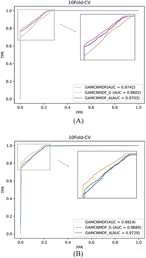
The ROC curves of GAMCNMDF, GAMCNMDF_A and GAMCNMDF_G on database HMDD v2.0 (A) and database HMDD v3.2 (B).
Small molecule–miRNA associations prediction
To show that GAMCNMDF works well in other datasets, we also applied our model to identify small molecules and miRNA associations. We utilized a dataset consistent with a prior investigation [33], encompassing 831 small molecules, 541 miRNAs and a set of 664 established associations. Based on this dataset, we employed 5-fold cross-validation and compared our result with the bounded nuclear norm regularization model (BNNRSMMA) [33], the triple layer heterogeneous network model (TLHNSMMA) [34], the graphlet interaction model (GISMMA) [35], the Sparse Learning and Heterogeneous Graph model (SLHGISMMA) [36] and the network model (SMiR-NBI) [37]. As shown in Figure 4, our model also performs well, providing further evidence that GAMCNMDF has a good generalization ability.
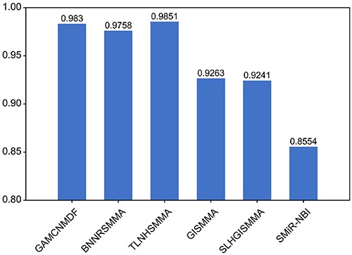
Comparison with other methods on a small molecule–miRNA dataset by 5-fold CV.
Experiment settings
In this study, we considered several hyperparameters that have an impact on the prediction results. For the similarity fusion step, we followed a previous study [23] and set the parameter |$k$| in the KNN to |$N/10$|, and |$N$| represents the total count of nodes present in the similarity network. As a result, we set |$\text{k}{\text{m}}$| to 55 and |$\text{k}{\text{d}}$| to 33 for miRNA similarity fusion and disease similarity fusion. The hidden layer of the generative adversarial matrix completion model utilized the Rectified Linear Unit (ReLU) activation function in the complete neural network. The units in the hidden layer were adjusted based on the database under consideration, with 878 units for one database and 1162 units for another.
Case studies
To further assess whether GAMCNMDF could perform well in terms of proof of ability to make inferences, we selected lung neoplasms and gastric neoplasms as case studies using dbDEMC v2.0 [38] and miRCancer [39]. We trained the GAMCNMDF model based on the dataset obtained on the database HMDD v2.0, removed known associations, prioritized all relevant miRNAs for the studied diseases according to GAMCNMDF’s prediction results and finally conducted validation against two well-established MDA databases by picking out the 50 most relevant miRNAs. In Table 4, 49 of the top lung cancer-associated 50 miRNAs are all confirmed. As shown in Table 5, we further performed predictions on miRNAs associated with gastric cancer and subsequently verified the top 48 miRNAs using the aforementioned two databases. More specifically, expression levels of hsa-mir-144 are generally lower in lung cancer cells and higher in normal lung tissue. hsa-mir-144 may regulate these lung cancer biological functions by directly targeting several related genes [40]. hsa-mir-647 expression was significantly downregulated in gastric cancer tissues, targeting multiple signaling pathways associated with gastric cancer [41, 42]. miR-381 has been found to exert oncogenic effects in gastric cancer cells, including promoting cell proliferation, invasion and migration, as well as suppressing apoptosis. These effects are mediated through its direct targeting of PTEN (phosphodiesterase and tensin inhibitors) proteins [43].
The top 50 potential miRNAs associated with lung neoplasms.( I, II denote dbDEMC,miRCancer)
| Rank | miRNA | Evidence | Rank | miRNA name | Evidence |
|---|---|---|---|---|---|
| 1 | hsa-mir-144 | I, II | 26 | hsa-mir-449a | I, II |
| 2 | hsa-mir-105-1 | I | 27 | hsa-mir-550a-2 | I |
| 3 | hsa-mir-151b | I | 28 | hsa-mir-378b | I |
| 4 | hsa-mir-4257 | I | 29 | hsa-mir-571 | I |
| 5 | hsa-mir-125b-2 | I, II | 30 | hsa-mir-409 | I |
| 6 | hsa-mir-1293 | I | 31 | hsa-mir-550b-1 | I |
| 7 | hsa-mir-378d-1 | I | 32 | hsa-mir-519d | I |
| 8 | hsa-mir-617 | I | 33 | hsa-mir-298 | I |
| 9 | hsa-mir-378c | I | 34 | hsa-mir-616 | I, II |
| 10 | hsa-mir-1254-1 | I, II | 35 | hsa-mir-133a-2 | I, II |
| 11 | hsa-mir-621 | I | 36 | hsa-mir-513c | I |
| 12 | hsa-mir-320b-1 | I | 37 | hsa-mir-23b | I, II |
| 13 | hsa-mir-1285-2 | I | 38 | hsa-mir-3179-3 | I |
| 14 | hsa-mir-378e | I | 39 | hsa-mir-612 | I |
| 15 | hsa-mir-3186 | I | 40 | hsa-mir-3940 | I, II |
| 16 | hsa-mir-590 | I, II | 41 | hsa-mir-492 | I |
| 17 | hsa-mir-658 | I | 42 | hsa-mir-520e | I |
| 18 | hsa-mir-608 | I | 43 | hsa-mir-339 | I, II |
| 19 | hsa-mir-582 | I, II | 44 | hsa-mir-1302-5 | unconfirmed |
| 20 | hsa-mir-320c-1 | I | 45 | hsa-mir-941-3 | I |
| 21 | hsa-mir-1915 | I | 46 | hsa-mir-361 | I, II |
| 22 | hsa-mir-1183 | I | 47 | hsa-mir-320a | I, II |
| 23 | hsa-mir-328 | I, II | 48 | hsa-mir-506 | I, II |
| 24 | hsa-mir-154 | I, II | 49 | hsa-mir-296 | I, II |
| 25 | hsa-mir-1273a | I | 50 | hsa-mir-500b | I |
The top 50 potential miRNAs associated with gastric neoplasms( I, II denote dbDEMC,miRCancer)
| Rank | miRNA | Evidence | Rank | miRNA name | Evidence |
|---|---|---|---|---|---|
| 1 | hsa-mir-647 | I, II | 26 | hsa-mir-769 | I |
| 2 | hsa-mir-505 | I, II | 27 | hsa-mir-642b | I |
| 3 | hsa-mir-381 | I, II | 28 | hsa-mir-490 | I, II |
| 4 | hsa-mir-522 | I | 29 | hsa-mir-1302-8 | unconfirmed |
| 5 | hsa-mir-598 | I, II | 30 | hsa-mir-23b | I, II |
| 6 | hsa-mir-612 | I | 31 | hsa-mir-592 | I, II |
| 7 | hsa-mir-498 | I, II | 32 | hsa-mir-133a-1 | I |
| 8 | hsa-mir-590 | I, II | 33 | hsa-mir-630 | I, II |
| 9 | hsa-mir-365a | I | 34 | hsa-mir-30e | I, II |
| 10 | hsa-mir-96 | I | 35 | hsa-mir-583 | I |
| 11 | hsa-mir-362 | I, II | 36 | hsa-mir-521-2 | I |
| 12 | hsa-mir-648 | I | 37 | hsa-mir-323b | I |
| 13 | hsa-mir-548a | unconfirmed | 38 | hsa-mir-942 | I |
| 14 | hsa-mir-548b | I | 39 | hsa-mir-628 | I |
| 15 | hsa-mir-520f | I, II | 40 | hsa-mir-1234 | I |
| 16 | hsa-mir-297 | I | 41 | hsa-mir-507 | I |
| 17 | hsa-mir-765 | I | 42 | hsa-mir-190a | I |
| 18 | hsa-mir-338 | I, II | 43 | hsa-mir-1275 | I, II |
| 19 | hsa-mir-708 | I, II | 44 | hsa-mir-1296 | I, II |
| 20 | hsa-mir-367 | I, II | 45 | hsa-mir-193a | I, II |
| 21 | hsa-mir-154 | I, II | 46 | hsa-mir-339 | I, II |
| 22 | hsa-mir-1260a | I | 47 | hsa-mir-512-1 | I |
| 23 | hsa-mir-642a | I | 48 | hsa-mir-205 | I, II |
| 24 | hsa-mir-758 | I | 49 | hsa-mir-181d | I, II |
| 25 | hsa-mir-211 | I, II | 50 | hsa-mir-1915 | I |
In addition, we downloaded miRNAseq data related to lung cancer and gastric cancer and compared the differential expression of miRNAs predicted by our model on these diseases, and our model’s predictions of miRNAs were further supported by the observation of differential expression in the corresponding diseases. This provides additional validation for the effectiveness of our model. The differential expression results are visually represented in Figure 5.
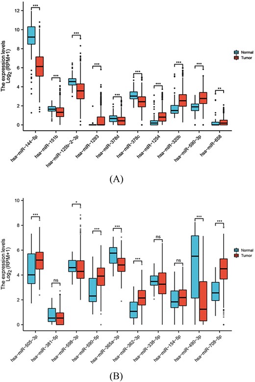
The results of the miRNA differential expression. (A) Ten predicted miRNAs for lung neoplasms. (B) Ten predicted miRNAs for gastric lung neoplasms.
CONCLUSION
Predicting the MDAs has been an essential task and the identification of disease-causing miRNA molecules is important for elucidating disease mechanisms, drug development and principles of personalized therapy. Given the limitations of biological experimental techniques, computational methods have become effective aids. In this study, we put forward GAMCNMDF to catch the latent MDAs. Not only do we introduce multiple sources of information but we also further improve prediction performance via adding ‘hints’ to ensure that the generator produces samples that closely resemble the actual underlying data distribution. We compared GAMCNMDF with other methods and demonstrate its superior performance; the cases of two diseases corroborate the effectiveness of GAMCNMDF. Moreover, GAMCNMDF identified small molecule–miRNA associations and further demonstrated its ability. In addition, there is room for improvement in the GAMCNMDF model, and further research is needed. For example, disease similarity contains only two types of information. The integration of more valid data sets will certainly bring great advances for future research. Given the increasing availability of incomplete, noisy, unreliable and inconsistent miRNA and disease-related biological data from various sources, the integration of heterogeneous data into a cohesive framework is a pressing research area. Future studies aim to address this challenge by exploring deep learning techniques [44–46] that enable the handling of multimodal data, leading to the enhanced prediction accuracy of computational methods. Moreover, with the aforementioned data, numerous computational prediction methods have emerged to identify potential MDAs. However, every approach exhibits its unique set of advantages and limitations, making it difficult to combine them effectively by analyzing their characteristics or developing simplified models to enhance prediction performance. Addressing these challenges will be a focus of our future research endeavors, as we aim to incorporate the aforementioned considerations into our work.
GAMCNMDF incorporated multi-omics data and constructed a heterogeneous miRNA disease network with a matrix representing it.
Unlike standard GANs, GAMCNMDF provided some additional information to the discriminator in the form of a ‘hint’ that further improved prediction accuracy.
GAMCNMDF imposed constraints on all the predicted values within a specific interval in the final matrix.
GAMCNMDF achieved great modeling results in predicting molecule–miRNA associations, demonstrating its strong generalization ability.
ACKNOWLEDGMENTS
This work is supported in part by funds from National key research and development plan sub-project (2021YFA10000102-3 and 2021YFA1000102-5), and the National Natural Science Foundation (Nos. 61873281, 61902430).
DATA AVAILABILITY
Code of GAMCNMDF and datasets are available at https://github.com/melodylyy/GAMCNMDF.
Author Biographies
Shu-Dong Wang received the PhD degree in control science and control engineering from Huazhong University of Science and Technology in 2004. She has been teaching in China University of Petroleum (East China) since 2014. Current research interests include biometrics, systems biology, the theory and application of DNA computational model.
Yun-Yin Li is a Master student of College of Computer Science and Technology, Qingdao Institute of Software, China University of Petroleum (East China), Qingdao, China. Her research interests include bioinformatics and machine learning.
Yuan-Yuan Zhang received the B.S. and M.S. degrees from the Shandong University of Science and Technology, in 2008 and 2011, respectively, and the PhD. degree from Xidian University, Xi’an, China, in 2016. She is currently an associate professor at the School of Information and Control Engineering, Qingdao University of Technology. Her research interests include computational bioinformatics, graph neural network and network representation learning.
Shan-Chen Pang received the PhD. degree in computer software and theory from the Tongji University, Shanghai, China, in 2008. He is currently a Professor and Ph.D. Supervisor with the China University of Petroleum (East China), Qingdao, China. His research interests include (advanced) Petri net theory and applications, formal methods, model checking, artificial intelligence, distributed concurrent system analysis and verification and other fields of teaching and research work.
Si-Bo Qiao is a PhD student of College of Computer Science and Technology, Qingdao Institute of Software, China University of Petroleum (East China), Qingdao, China. His research interests include bioinformatics and machine learning.
Yu Zhang is a Master student of College of Computer Science and Technology, Qingdao Institute of Software, China University of Petroleum (East China), Qingdao, China. Her research interests include bioinformatics and machine learning.
Fu-Yu Wang is a Master student of College of Computer Science and Technology, Qingdao Institute of Software, China University of Petroleum (East China), Qingdao, China. His research interests include bioinformatics and machine learning.
