


Abstract
Factor analysis, ranging from principal component analysis to nonnegative matrix factorization, represents a foremost approach in analyzing multi-dimensional data to extract valuable patterns, and is increasingly being applied in the context of multi-dimensional omics datasets represented in tensor form. However, traditional analytical methods are heavily dependent on the format and structure of the data itself, and if these change even slightly, the analyst must change their data analysis strategy and techniques and spend a considerable amount of time on data preprocessing. Additionally, many traditional methods cannot be applied as-is in the presence of missing values in the data. We present a new statistical framework, unified nonnegative matrix factorization (UNMF), for finding informative patterns in messy biological data sets. UNMF is designed for tidy data format and structure, making data analysis easier and simplifying the development of data analysis tools. UNMF can handle a wide range of data structures and formats, and works seamlessly with tensor data including missing observations and repeated measurements. The usefulness of UNMF is demonstrated through its application to several multi-dimensional omics data, offering user-friendly and unified features for analysis and integration. Its application holds great potential for the life science community. UNMF is implemented with R and is available from GitHub (https://github.com/abikoushi/moltenNMF).
INTRODUCTION
The utilization of multi-dimensional omics technologies is becoming increasingly ubiquitous in all aspects of life science. As an illustration, data such as genome, epigenome, transcriptome, proteome and metabolome can be quantified under varying conditions and at different times, in order to unveil associations between genotype and environmental factors [1]. These diverse forms of biological information can be represented through the use of multi-dimensional arrays, formally referred to as tensors.
Factor analysis is a premier approach for analyzing multi-dimensional data to extract useful patterns and is increasingly being applied in the context of multiomics datasets. This model class encompasses a broad range of analytical methods including principal component analysis to nonnegative matrix factorization. Recently, it has been expanded to model various structures of datasets such as multiple data modalities, sample group structures and temporal or spatial structures [2–4]. Nevertheless, conventional methods are strongly dependent on the format and structure of the data and require modification of analytical strategies and techniques, as well as a significant amount of time spent on data cleaning and preprocessing, when any of these are altered even slightly. Furthermore, many traditional methods cannot be directly applied when the data contain missing values.
In this study, our objective is to address these issues and introduce a novel statistical methodology, named unified nonnegative matrix factorization (UNMF), to discover meaningful patterns in messy biological data sets. Our approach can be applied to multi-dimensional omics data, regardless of their format or structure, and is designed to comply with the principles of tidy data format and structure as recommended by [5]. The aim of our methodology is to simplify data analysis and streamline the development of data analysis tools that can be used cohesively.
The key contributions of our research are as follows:
(1) Our framework can handle a wide array of data structures and formats in a unified manner, facilitating data analysis and allowing for the focus on identifying specific patterns of interest rather than handling uninteresting logistics of the data.
(2) Our model seamlessly works with tensor data that encompass missing observations and repeated measurements, even sparse ones, which would pose challenges for traditional approaches.
(3) We have developed a straightforward and efficient learning procedure of UNMF using variational Bayes and derived a lower bound on marginal likelihood (evidence lower bound; ELBO).
To highlight the usefulness of UNMF, we provide examples of its application to several multi-dimensional omics data. UNMF provides user-friendly and unified features to analyze and integrate multi-dimensional omics data and its application holds great potential for the life science community.
The structure of this paper will proceed as follows. In the ‘Conceptual View’ section, we will discuss in detail why UNMF is not restricted on the formats of the data and how it can be used for predictions and explanations. The ‘Model and variational inference’ section describes the generative model and its learning procedure. The ‘Results’ section contains two sub-section. Firstly, we conduct simulation study to show the behavior of the our estimator. Next, we analyze the more realistic dataset of metagenomics and RNA sequencing.
CONCEPTUAL VIEW
Traditional factor analysis techniques such as principal component analysis [6], nonnegative matrix factorization [7] and latent Dirichlet allocation [8] seek to find matrices |$Z$| and |$W$| such that |$Y \approx ZW$|, given a data matrix |$Y$|. Here, each row of the matrix |$Z$| represents latent variables that describe the structure and characteristics of data, corresponding to |$k$| representative patterns inherent in the data. Additionally, each row of the matrix |$W$| describes the relationship between latent factors and observed variables through a linear mapping. Factor analysis is a powerful approach for extracting valuable patterns in multi-dimensional data, but conventional traditional factor analysis is heavily dependent on the structure and format of the data matrix, rendering them inapplicable when the matrix contains missing values or lacks a clear form.
Unlike existing factor analysis techniques for multi data, UNMF takes in tidy data [5, 9] as input, which is a data format that is coherent in structure and meaning and satisfies the following conditions:
(1) Each variable forms one column.
(2) Each observation forms one row.
(3) The type of observational unit for each observation forms one table.
(4) Each value constitutes one cell.
Figure 1 shows an example of the traditional matrix format and tidy data format using toy data. When adding additional observations to the data set, tidy data format simply requires adding columns, while the normal matrix format requires expanding the multi-dimensional array. Similarly, in the case of missing values, tidy data format only requires deleting rows, while the normal matrix format requires some form of imputation to fill in the missing values for factor analysis.
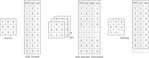
Visual example of the tidy format. The ‘matrix’ and the ‘tidy’ format have the same information. The gray parts of the ‘tidy’ format can be regarded as explanatory variables.
UNMF performs factorization of input data in a manner akin to traditional factor analysis, decomposing them into latent factors, and embeds the samples in a lower dimensional latent space. Simultaneously, UNMF employs linear mapping to establish the relationship between the latent factors and observed variables. Given data matrices represented in tidy data format and a vector of observed data values denoted by |$y=(y_1,\ldots , y_N)^{\prime}$| and a matrix |$X=(x_{nd})$| (|$x_{nd} \in \{0,1\}$|) representing structure and meaning, UNMF finds a nonnegative value matrix |$V$| of |$D \times L$| such that
Here |$D$| is determined by dimension (number of columns) of |$X$| and |$L$| is a user-specified parameter. A larger |$L$| makes the model more expressive but can also lead to overfitting. The matrix |$V$| describes the co-occurrence relationships of |$y_n$|, and if the vectors |$v_n = (\prod _{d} v_{d1}^{x_{nd}}, \ldots , \prod _{d} v_{dL}^{x_{nd}})$| characterized by non-zero elements of the explanatory variable |$X$| are similar in direction, |$y$| will have higher values.
An example of matrix factorization in tidy data format using UNMF is shown in Figure 2. Suppose an experiment using two subjects yields observations of three features and the second subject has a missing value for the third feature which are represented by a matrix |$Y$|. The tidy data format of the matrix |$Y$| can be represented using a vector |$y$| and a matrix |$X$|. Here, the indicator |$i$| represents the sample, the indicator |$j$| represents the feature and the indicator |$h$| represents the number of rows in the tidy data. In the tidy data format, the index of |$y_{nk}$| is represented by the explanatory variable shown in the following equation. |$X$| represents a one-hot vector that indicates the rows and columns of matrix |$y_{nk}$|. For instance, the subscripts |$(n,k)=(1,1)$| and |$(n,k)=(2,1)$| of matrix |$Y$| correspond to the first and second row vectors |$x_1=(1,0,1,0,0)$| and |$x_2=(0,1,1,0,0)$| of matrix |$X$|. It should be noted here that the information content of the two data formats does not change.
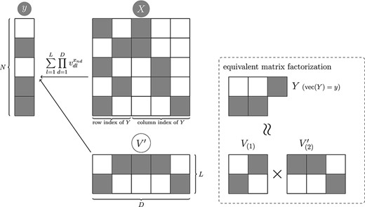
Visual example to understand the equation 1. The gray circles indicate observed variables, and white indicates latent variable.
UNMF performs factorization of input data represented in tidy data format in a manner similar to traditional factor analysis and approximates it as in the following equation:
where |$V_{(1)} = (\prod _{d=1}^2 v_{dl}^{x_{nd}})$| and |$(V_{(2)} = \prod _{d=3}^4 v_{dl}^{x_{nd}})$|.
UNMF also deals with cases where subjects who are observed in the first instance are not observed in the second instance, meaning that the data contain missing values. When such data are held as a tensor, they require special processing, such as imputation, in order to perform factor analysis due to the existence of missing values at the second point in time. UNMF is capable of handling such missing data in a natural manner. If the subject does not exist at the second point in time, the equivalent row does not exist in the organized data and there is no hindrance in building the model. Conversely, even if there are duplicates in the data, the same result is outputted.
MODEL AND VARIATIONAL INFERENCE
UNMF is formalized within a probabilistic framework as follows:
The gamma prior is easy to compute, and it constrains the value of |$v_{dl}$| to be nonnegative, making it easier to interpret. Simply, higher values of |$v_{dl}$|s have highly co-occurrences.
Equation 2 is equivalent to the following:
Using the mean field assumption [10], we introduce variational Bayesian inference updates for the proposition model with the objective of finding the variational posterior distribution of the latent variable |$q(v_{dl})$|.
For any latent variable, say |$w$|, let |$\tilde w$| be the mean of |$w$| evaluated by the variational posterior. i.e.
Note that |$\widetilde{\log w} = \int \log w q(w) \, dw$| is not equal to |$\log (\tilde{w})$|, in general. The variational posterior of |$u_{nl}$| is expressed as a multinomial distribution, and the updates for |$u_{nl}$| are defined by |$\widetilde{u_{nl}}= y_{n} r_{nl}$|, where |$r_{nl}$| is denoted as
The variational posterior |$q(v_{dl})$| is characterized as a gamma distribution with shape parameter |$\hat a_{dl}$| and rate parameter |$\hat b_{dl}$|, as outlined in
To summarize, the following steps outline the proposed procedure:
Initialize |$v_{dl}$| through a gamma distribution.
Repeat the following two steps at a specified iteration number:
– Update |$\widetilde{u_{nl}}$| using Equation 4.
Update |$\widetilde{v_{dl}}$| and |$\widetilde{\log v_{dl}}$| using Equation 5.
The convergence of this algorithm is substantiated by the lower bound of the marginal likelihood (sometimes referred as evidence lower bound; ELBO), say |$\mathcal{L}(q)$|, to monitor the convergence of the algorithm,
where |$\theta $| is all of the variational parameters, and |$\boldsymbol{y}=(y_1, \ldots , y_N)^{\prime}$|.
After some manipulations, the following expression is obtained:
where |$R_n= \sum _{l=1}^{L} \exp ( x_{nd}\widetilde{\log v_{dl}})$|
Our procedure of the variational inference can be regarded as finding the |$q(\theta )$| such that maximizing Eq.6.
Discrete probability distributions beyond the Poisson model
In prior sections, we delved into the Poisson distribution model; however, the multinomial distribution is also frequently employed as a fundamental discrete probability distribution. The multinomial distribution is utilized when there is an upper limit on the data’s values. Moreover, in cases of over-dispersion of the data, the negative binomial distribution is often used. Despite the fact that Poisson distribution serves as the foundation for these distributions, our model can be applied to a range of count data.
For instance, we consider the data generation process of Latent Dirichlet Allocation (LDA) [11]:
The marginal distribution of |$Y_n$| is
Now, If we let |$\eta _n =\lambda _n W_n$| and consider the problem of estimating |$\eta _n$|, then NMF is equivalent to LDA. In order to evaluate the relative magnitude of the values, we can normalize the estimated |$\eta _n$| at post hoc.
Additionally, with a simple alteration to the model, the negative binomial distribution can also be employed:
The variational posterior of |$v_{dl}$| is
where the shape and rate parameters are, respectively,
The variational posterior of |$z_{n}$| is
The hyperparameter |$\tau $| can be optimized through the application of Newton’s method [10].
RESULUTS
Simulation Study
We performed three simulations to evaluate the precision of estimation in the UNMF framework.
(1) We generated synthetic data in accordance with the model’s assumptions and contrasted the result with the expectation a posteriori (EAP). The consistency of the estimator was demonstrated through this evaluation.
(2) Synthetic data were generated and the optimal number of components, |$L$|, was selected through holdout validation. The behavior of validation-loss was then analyzed.
(3) Synthetic data were produced using LDA’s model and compared with the EAP, demonstrating the robustness of the estimator.
The mean and standard deviation of estimators were assessed in the first scenario. Synthetic data were generated using |$N=100 \times 100 \times 3$| samples and observations were performed. The parameters |$v_{dl}$| were randomly drawn from a gamma distribution with shape parameter |$a=1$| and rate parameter |$b=0.1$|, while the parameters |$W$| were generated from a gamma distribution with parameters |$a=1$| and rate parameter |$b=0.01$|. The comparison between the true parameters and the mean and standard deviation of estimates obtained from 100 simulations is depicted in Figure 3. We observed that the points were arranged diagonally, indicating that the estimator was small biases.
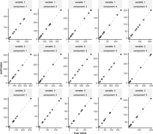
The comparison true parameters and the mean of estimated parameters. The error bars indicates standard deviation.
Subsequently, in the second scenario, we evaluate the model selection log-likelihood as calculated on the test data. The parameters and data are generated in the same manner as previously described in each simulation. From 1000 trials, it was observed that |$L = 5$| was selected 644 times (Figure 4).
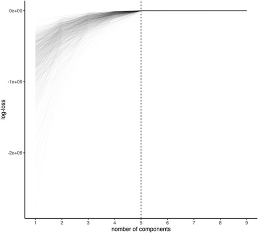
Log-likelihood evaluated at test data. One line corresponds to one synthetic dataset.
In the third scenario, a nonnegative integer matrix |$Y$| (|$100 \times 100$|) is generated from a multinomial distribution, while |$W_n$| and |$H_l$| are randomly drawn from a Dirichlet distribution with all parameters equal to 2. This demonstrates that the proposed method yields credible estimations (Figure 5). These simulation studies indicate that UNMF has consistency. This property helps interpretation of estimated |$V$|. If the optimal points of the parameters are not substantially unique, the obtained estimates have potentially multiple interpretations. If the analyst presents only one of them, the results can be misleading. With this validation, it is feasible to apply the method to real data to determine its compatibility with existing studies.
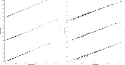
Estimated |$v_{dl}$| versus |$H_{lk}$| and |$W_{nl}$| (true value). The points indicate mean, and the error bars indicate standard deviation.
Selected number of component |$L$| by holdout validation (true is 5)
| |$L$| | 5 | 6 | 7 | 8 | 9 |
|---|---|---|---|---|---|
| 0.64 | 0.21 | 0.06 | 0.04 | 0.03 |
| |$L$| | 5 | 6 | 7 | 8 | 9 |
|---|---|---|---|---|---|
| 0.64 | 0.21 | 0.06 | 0.04 | 0.03 |
Selected number of component |$L$| by holdout validation (true is 5)
| |$L$| | 5 | 6 | 7 | 8 | 9 |
|---|---|---|---|---|---|
| 0.64 | 0.21 | 0.06 | 0.04 | 0.03 |
| |$L$| | 5 | 6 | 7 | 8 | 9 |
|---|---|---|---|---|---|
| 0.64 | 0.21 | 0.06 | 0.04 | 0.03 |
Real data analysis
Metagenomic sample analysis
In this section, we conduct two metagenomic sample analysis, examining the data from David et al. [12] and Kostic et al. [13]. The analysis is performed using the abundance of genus-level taxa.
Prior to showing the analysis results, we establish certain quantity to help interpretation.
FLEX, which stands for Frequency-Expectation [14], is defined as the harmonic mean of two probabilities, with the first term representing the probability of microbe |$j$| given component |$k$| and the second representing the exclusive presence of microbe |$j$| in component |$k$|.
Now, we undertake an analysis of David’s data. David and his colleagues conducted a longitudinal study of fecal metagenomes from two donors, A and B. However, for the purposes of this analysis, we shall limit our focus solely to donor B. This decision was made as both donors are not representative samples. The data reveal that donor B had an episode of enteric infection between Days 151 and 159. The information is accessible via the R package ‘themetagenomics’ (https://github.com/EESI/themetagenomics). For donor B, 530 species of bacteria (unknown species were aggregated as ‘unknown”) were recorded at 176 time points.
In order to determine the optimal number of components |$L$|, we employed a holdout validation approach and evaluated the log-likelihood at the test data. A randomly selected 10% of the data was designated as test data, with the remainder serving as training data. The values of log-likelihood are illustrated in Figure 6. Figure 7 displays the estimates of |$v_{dl}$| for each day, with a marked increase in component 4 around Days 150–160. In Figure 8, we depict the representative microbes for each component based on the top 10 FLEX values. Component 4 is characterized by the genera Eshtishia/Shigella, Salmonella and Clostridium, which are known to cause food poisoning.
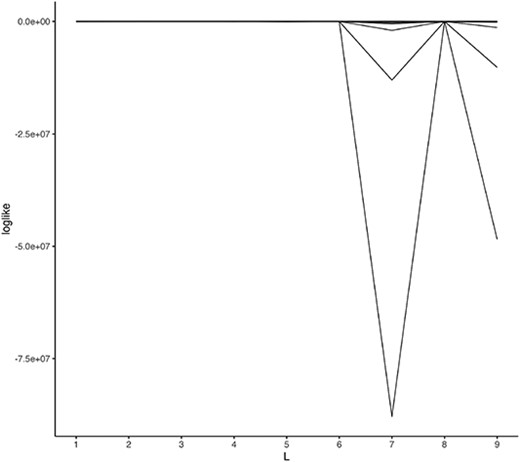
Log-likelihood evaluated at test data. Each line corresponds one data point.
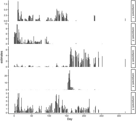
x-axis: time point, y-axis: estimates of |$v_{dl}$|.
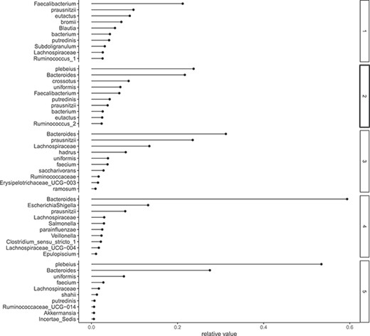
Relative frequency. x-axis: estimates of |$v_{dl}$|, y-axis: species corresponds |$d$|.
Subsequently, we analyze Kostic’s data. Kostic and colleagues conducted research on the correlation between type 1 diabetes (T1D) and metagenome by cohort. This information can be accessed at https://pubs.broadinstitute.org/diabimmune/t1d-cohort/resources/16s-sequence-data. The data included a total of 19 unique subjects, eight, seven and four in control, seroconverted and T1D, respectively. This study is a cohort study spanning Days 42 to 1233 of life and includes repeated measures for subjects. Since subjects are not sampled at the same age and the number of repeats is also different, these data require specific preprocessing to be handled by ordinary matrix factorization. However, UNMF does not require any specials. Our explanatory variables, denoted as |$X$|, consist of age, subject id, bacterial species and T1D status (control, T1D and seroconversion). We label the model containing T1D status information as model 1, and the model without it as model 0.
As illustrated in Figure 2, the log-likelihood value assessed by holdout-validation indicates that the optimal number of components is |$L=2$|. Nonetheless, null models (excluding T1D status) reveal greater likelihoods in the test data, as shown in Table 2. Consequently, the association between T1D and the enteric microbiome cannot be deemed credible. As a side note, the log-likelihood of the test data for model 1 at |$L=5$| is very small due to overfitting (Table 2).
The mean of log-likelihood evaluated at test data.
| |$L$| | 1 | 2 | 3 | 4 | 5 |
|---|---|---|---|---|---|
| model 0 | −821.95 | −749.25 | −894.72 | −1221.73 | −1627.17 |
| model 1 | −822.14 | −785.38 | −867.18 | −1076.71 | −385328.61 |
| |$L$| | 1 | 2 | 3 | 4 | 5 |
|---|---|---|---|---|---|
| model 0 | −821.95 | −749.25 | −894.72 | −1221.73 | −1627.17 |
| model 1 | −822.14 | −785.38 | −867.18 | −1076.71 | −385328.61 |
The analysis should proceed using model 1, which assumes a relationship between T1D and the gut microbiome. Kostic et al. proposed that individuals with T1D exhibit decreased alpha-diversity in their gut microbiome. This finding is consistent with the entropy distribution (refer to Table 3).
Entropy when the microbe are multinomial distributed
| control | seroconverted | T1D |
|---|---|---|
| 2.49 | 2.24 | 2.35 |
| control | seroconverted | T1D |
|---|---|---|
| 2.49 | 2.24 | 2.35 |
Entropy when the microbe are multinomial distributed
| control | seroconverted | T1D |
|---|---|---|
| 2.49 | 2.24 | 2.35 |
| control | seroconverted | T1D |
|---|---|---|
| 2.49 | 2.24 | 2.35 |
Lastly, Figure 10 illustrates the estimates of |$v_{dl}$| for each age group. It indicates that component 2 experiences growth after about 1000 days, and a negative correlation exists between components 1 and 2. When utilizing model 1, the findings obtained align with the report put forth by [13], as previously described. It is important to note, however, that these results were achieved under the presumption of a relationship between T1D and the gut microbiome. As T1D information does not contribute to enhancing the prediction accuracy, we cannot make a compelling argument for the existence of said association. In general, when preprocessing involves multiple steps such as normalization, smoothing and missing data imputation, the resulting analysis possesses a significant number of degrees of freedom, rendering validation a more complex undertaking. As demonstrated in this section’s analysis, hypothesis verification is straightforward owing to the ability of UNMF to generate predictions and interpretations within a single model.
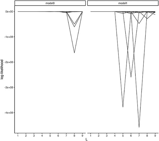
Log-likelihood evaluated at test data. Each line corresponds one data point.
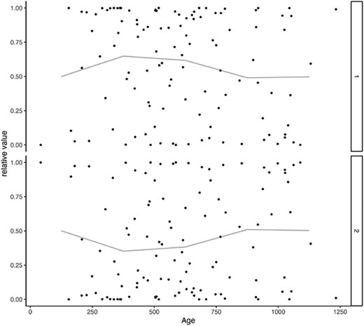
x-axis: age (daily), y-axis: estimates. The lines indicate mean of each 250.
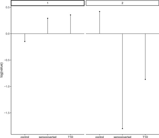
x-axis: T1D status, y-axis: corresponds estimates of |$v_{dl}$|.
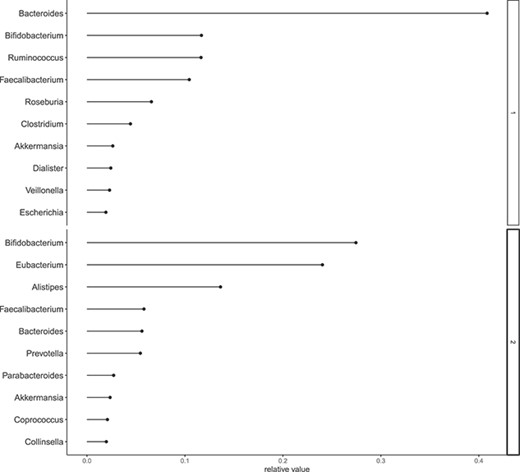
Relative frequency. x-axis: estimates of |$v_{dl}$|, y-axis: species corresponds |$d$|.
Gene expression analysis
Revealing the gene expression responses to drugs leads to the knowledge about drug discovery. However, due to the large number of combinations of conditions such as cells, genes and drug doses, there are many missing values in the gene expression data for drug response. Therefore, missing values imputation in drug response gene expression data is needed.
An illustration of missing data completion is demonstrated through analyzing gene expression profiles (GSE92742, [15, 16]) obtained from the Gene Expression Omnibus database (GEO; [17]). The analysis encompasses ‘level 2’ data, consisting of 1246 landmark genes, with expression levels recorded at 6, 24, 96, 120, 144 and 168 hours post-treatment. Three cell types (MCF7, PC3 and VCAP) were treated with dosages of 0, 25ul, 10 and 30 um. Gene expression profiling often results in missing values, and the aim of this analysis is to predict these missing parts.
To assess the performance of missing data completion, artificial missing values were introduced to the original data. The conditions under which records were deleted were randomly selected, resulting in training data lacking observations with the same four conditions (dose, time-point, marker gene and cell) as the test data.
The prediction of missing values was compared with XGboost [18] as the baseline method. XGBoost and its analogue, ensemble models based on decision trees, have been reported to have excellent performance in predicting tabular data [19]. Both UNMF and XGBoost were applied on tidy formatted data to predict gene expressions with the same explanatory variables (above-mentioned four conditions). The comparison, presented in Figure 13, showcases the prediction against the observed (true) values, with root mean squared errors (RMSEs) of 820 (left panel) and 1300 (right panel), respectively. Note that the mean and standard deviation for the entire data are 2228.463 and 1617.54, respectively (the range is |$[1, 25465]$|), so this RMSE is not too large. The GSE data were resampled to 10 million rows, with 1 million conditions designated as test data and the remaining as training data.
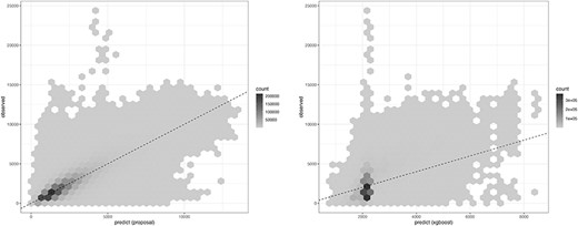
Comparison of the prediction. x-axis: predicted, y-axis: observed (true value).
Table 4 illustrates that the results across varying hyperparameter choices display a consistent trend.
Comparison of the prediction. We resampled the GSE data to |$10^6$| rows, with |$10^5$| conditions as test data and the rest as training data.
| hyperparameter | (XGBoost) | |||
|---|---|---|---|---|
| eta | max_depth | lambda | alpha | RMSE |
| 0.30 | 6.00 | 1.00 | 0.00 | 1314.17 |
| 0.30 | 5.00 | 0.50 | 0.00 | 1340.58 |
| 0.50 | 15.00 | 0.50 | 0.10 | 1032.77 |
| 1.50 | 30.00 | 1.00 | 0.00 | 800.95 |
| (UNMF) | ||||
| L | RMSE | |||
| 2 | 816.67 | |||
| 3 | 780.11 | |||
| 4 | 762.93 | |||
| 5 | 763.50 | |||
Our method, UNMF, utilizes features constructed as products of multiple factors, allowing for the expression of their interactions in a natural manner. In a Bayesian perspective, the ensemble of multiple predictors corresponds to the posterior predictive, integrated through the posterior distribution, and the regularization term corresponds to the prior distribution. In Eq.6, the first line has a larger value at better fitting, and the next two lines are penalty for departing from the prior distribution. These factors make UNMF flexible while avoiding overfitting.
CONCLUSION
In this study, we introduced a novel statistical framework, known as UNMF, to extract meaningful patterns from complex biological data sets, without being restricted by the data’s format and structure. UNMF can handle a wide range of data structures and formats, and works seamlessly with tensor data including missing observations and repeated measurements.
In the metagenomic sample analysis, we demonstrated the effectiveness of the UNMF in knowledge discovery. In case-control studies, a crucial aspect is identifying differences between cases and controls. Our results, obtained from a metagenomic example, indicated that the UNMF can effectively perform this task, even when the data have a complex structure (subject |$\times $| time |$\times $| microbe |$\times $| case-control). Furthermore, the gene expression example demonstrated that the UNMF can perform reasonable predictions while maintaining interpretability. This property comes from the inference procedure and the non-negativity, as we have discussed in the ‘Model and variational inference’ and ‘Simulation study’ sections. These features make UNMF a potentially valuable tool for a wide range of analysis.
This research holds potential for future expansion and may make significant contributions to the field. As omics data encompass more than just count data, it may be worth considering the use of alternative distributions, such as normal or log normal, within the UNMF framework.
We believe that UNMF offers a user-friendly, unified functionality for analyzing and integrating multi-dimensional and multi-dimensional omics data, and its application holds great potential for the life sciences field.
Default prior distribution
We set the gamma prior distribution weakly informative [20] as not to rule out the information contained in data. This means, even if the observation has many 0s or outlier, numerical errors are not occurred, and otherwise provide similar result to the maximum likelihood estimator.
To check the sensitivity of proposed model, we analyze the four dataset (Titanic, HairEyeColor, UCBAdmissions and Lander, 2017’s National Election Study in 1964) which have different range of values. The data of ‘Titanic’, ‘HairEyeColor’ and ‘UCBAdmissions’ are included in the statistical software R as default.
We set |$a=0.1,0,2, \ldots , 0.9$| and |$b=10^0, 10^{-1}, \ldots , 10^{-4}$| as hyperparameters, respectively. Figure 14 shows the difference between maximum likelihood estimator and EAP. In all cases, the difference is close to 0 when |$a=0.05$| and |$b=0.01$|.
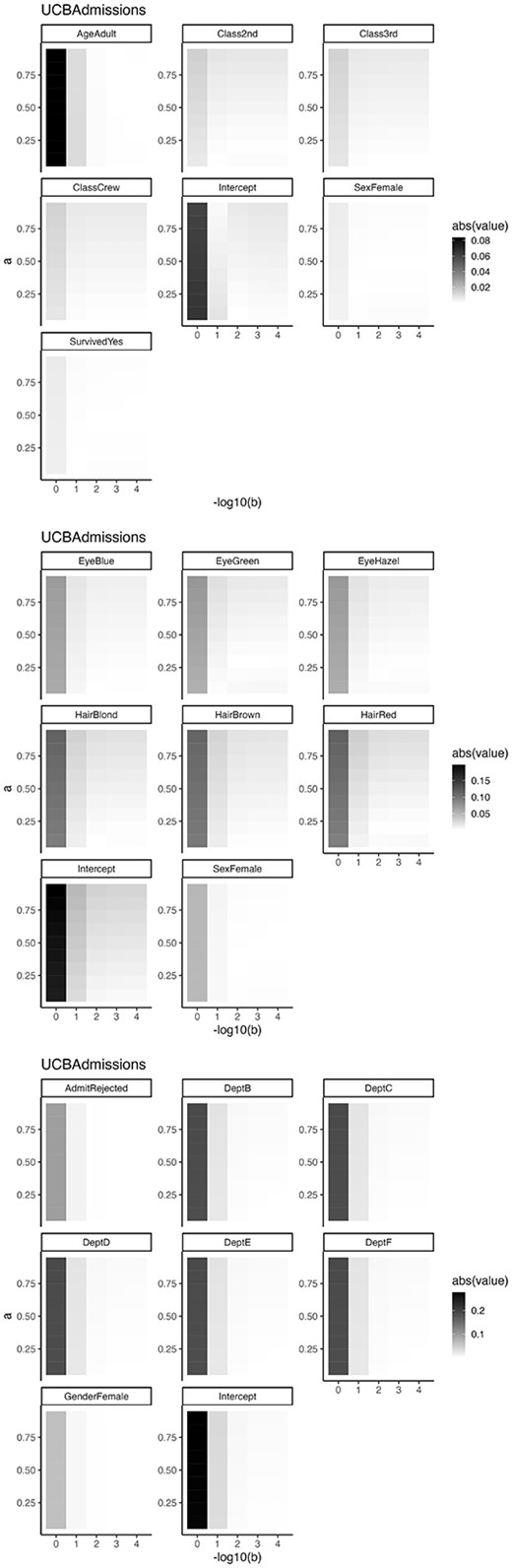
Absolute value of the difference between maximum likelihood estimator and EAP
Next, Figure 15 shows regression coefficients for National Election Study data. Our proposed estimator not occurred numerical divergent for variable `Raceblack' and other variables no drastic change from MLE.
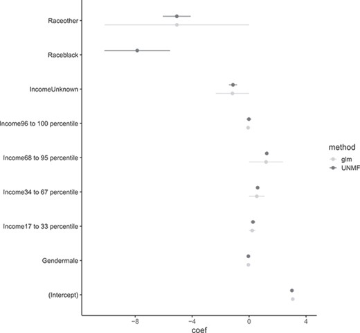
Comparison between maximum likelihood estimator and EAP. MLE about ‘Raceblack’ are divergent numerically.
This example illustrates our procedure gives reasonable estimates.
We develop a novel statistical framework, UNMF, to extract meaningful feature from biological data sets without being restricted by the data’s format and structure.
UNMF works seamlessly with tensor data including missing observations and repeated measurements.
UNMF achieves both predictive accuracy and model interpretability through nonnegative constraints and Bayesian procedures.
AUTHOR CONTRIBUTIONS STATEMENT
K.A. and T.S. developed the method and analyzed the results. K.A. conducted the simulation study. K.A. and T.S. wrote and reviewed the manuscript.
ACKNOWLEDGMENTS
This work was supported by grants from KAKENHI Grants-in-Aid for Young Scientists (A.K., grant number 20K19921), KAKENHI Grants-in Aid for Scientific Research (B) (T.S., grant number 20H04281), KAKENHI Grants-in-Aid for Scientific Research on Innovative Areas on Information Physics of Living Matters (T.S., grant number 22H04839), KAKENHI Grants-in-Aid for Challenging Exploratory Research (T.S., grant number 20K21832), KAKENHI Grant-in-Aid for Transformative Research Areas (platforms for Advanced Technologies and Research Resources) (T.S., grant number 22H04925), and KAKENHI Grant-in-Aid for Transformative Research Areas (A) (T.S., grant number 23H04938) from the Japan Society for the Promotion of Science (JSPS). It was also supported by RADDAR-J (T.S., grant number 22ek0109488), Project for P-PROMOTE (T.S., grant number 22ama221215 and 22ama221501), Brain/MINDS Health and Diseases (T.S., grant number 22wm0425007) from the Japan Agency for Medical Research and Development (AMED), and Moonshot R&D (T.S., grant number JPMJMS2025) from the Japan Science and Technology Agency (JST). The super-computing resource was provided by Human Genome Center (The University of Tokyo) and AI Bridging Cloud Infrastructure (ABCI) (National Institute of Advanced Industrial Science and Technology).
REFERENCES
