


Abstract
Nucleic acid-binding proteins are proteins that interact with DNA and RNA to regulate gene expression and transcriptional control. The pathogenesis of many human diseases is related to abnormal gene expression. Therefore, recognizing nucleic acid-binding proteins accurately and efficiently has important implications for disease research. To address this question, some scientists have proposed the method of using sequence information to identify nucleic acid-binding proteins. However, different types of nucleic acid-binding proteins have different subfunctions, and these methods ignore their internal differences, so the performance of the predictor can be further improved. In this study, we proposed a new method, called iDRPro-SC, to predict the type of nucleic acid-binding proteins based on the sequence information. iDRPro-SC considers the internal differences of nucleic acid-binding proteins and combines their subfunctions to build a complete dataset. Additionally, we used an ensemble learning to characterize and predict nucleic acid-binding proteins. The results of the test dataset showed that iDRPro-SC achieved the best prediction performance and was superior to the other existing nucleic acid-binding protein prediction methods. We have established a web server that can be accessed online: http://bliulab.net/iDRPro-SC.
INTRODUCTION
Nucleic acid-binding proteins (NABPs) are proteins that interact with DNA and RNA to regulate gene expression and transcriptional control [1–3]. The pathogenesis of many human diseases is related to abnormal gene expression. DNA-binding proteins (DBPs) include histones, helicases and transcription factors [4]. These proteins are involved in many important cellular activities, including gene transcription and regulation, single strand DNA binding and separation, chromatin formation and cell development. RNA-binding proteins (RBPs) interact with RNA as a special riboprotein complex, playing an important role in post-transcriptional gene regulation, alternative splicing, translation and the other gene expression processes [5]. NABPs are key regulators of gene expression, and thus better understanding of their functions can help improve understanding of the mechanisms of gene expression, the pathogenesis of various diseases and the discovery of therapeutic targets [6]. However, the time required and high cost of biochemical experiments limit the identification of NABPs, resulting in a huge gap between the number of known NABPs and that of NABPs to be studied.
Some scientists have proposed computational methods to identify NABPs. These methods can be divided into two categories depending on the different information used: structure-based methods and sequence-based methods. Although structure-based methods are usually more accurate than that sequence-based methods, only 0.36% of proteins in UniProtKB have structural information [7], which makes it unable to be widely used. We can divide sequence-based methods into three categories, including methods for identifying DBPs, methods for identifying RBPs and methods for simultaneously identifying DBPs and RBPs. For example, DNAbinder [8], StackDPPred [9] and DPP-PseAAC [10] are methods for predicting DBPs; SPOT-Seq-RNA [11], catRAPID [12], RNAPred [13], RBPPred [14], TriPepSVM [15] and DeepRBPPred [16] are methods for predicting RBPs; DeepDRBP-2L [17], iDBRP-ECHF [18] and IDRBP-PPCT [19] are methods for predicting DBPs and RBPs simultaneously. iDeepMV [20] uses several multi-view features to predict the RBPs. DeepDRBP-2L [17] is the first predictor to predict the DBPs, RBPs and DNA- and RNA- binding Proteins (DRBPs) by utilizing the convolutional neural network and long short-term memory (LSTM).
The above methods further promoted the identification of NABPs. However, almost all existing calculation methods ignore the fact that DBPs and RBPs have different functions [21]. For example, DBPs include activator proteins, developmental proteins and repressor proteins, and RBPs include ribonucleoproteins and rRNA-binding proteins. As shown in Figure 1, adding subfunction classifiers can easily divide the decision boundary, allowing for better distinction of different types of NABPs. Therefore, researchers should consider how to make better use of subfunction classifiers in the NABP task.
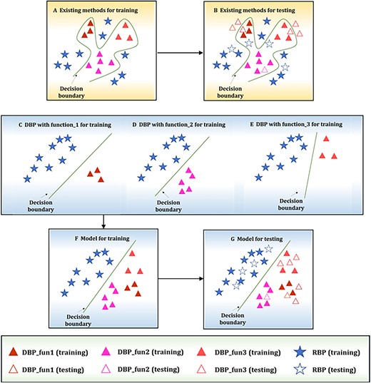
Illustration of the existing methods problems and the iDRPro-SC solution proposed in this study. (A) Training process of existing methods. (B) Testing process of existing methods. (C–E) Training process of different subfunction classifiers. (F) Training process of the ensemble model combining multiple subfunction classifiers. (G) Testing process of the ensemble model.
To solve the above problems, we propose a new method, called iDRPro-SC, to identify DBPs and RBPs. Compared with other existing NABP predictors, iDRPro-SC has the following advantages: (i) iDRPro-SC considers the subfunctions of NABPs to build a more complete dataset; (ii) iDRPro-SC takes into account the difference between DBPs and RBPs, which will be applied to the field of NABP identification. A comparison of iDRPro-SC with existing methods is shown in Figure 1
MATERIALS AND METHODS
Benchmark dataset
The benchmark dataset used in this study was previously described [17]. The benchmark dataset was derived exclusively from the Swiss-Prot database [22], which is a highly curated and reliable source of protein information. To identify DBPs and RBPs with specific functions, we used the Gene Ontology (GO) terms ‘DNA-binding’ (GO:0003677) and ‘RNA-binding’ (GO:0003723), respectively. The DRBPs were only those proteins annotated with the GO terms ‘DNA-binding’ (GO:0003677) and ‘RNA-binding’ (GO:0003723). We further ensured the reliability of the data by selecting proteins with manual evidence codes.
To accurately compare the performance of NABP predictors, the following two methods were used to construct the benchmark dataset: (a) a large number of DBPs and RBPs were added to the dataset to avoid overestimating the predictive values that only identify DBPs or RBPs, and (b) BLASTClust [23] was used to remove the redundancy of each type of protein in the benchmark dataset to ensure that the redundancy was no >35% [17]. Following previous studies [17], the benchmark dataset was expressed by the following formula:
After the above processing, the benchmark dataset contained 10 188 non-nucleic acid-binding proteins (NON-NABPs) and 11 875 NABPs. |${\mathbb{S}}_{NABP}$| included 7594 DBPs, 3948 RBPs and 333 DRBPs.
We searched for specific keywords in the Molecular function section of the Swiss-Prot database to identify proteins with specific functions, such as activator or repressor proteins. The keywords we used were KW-0010 for activator function and KW-0678 for repressor function. Considering that different proteins have different subfunctions, we further divided the |${\mathbb{S}}_{DBP}$| into |${\mathbb{S}}_{Activator}$|, |${\mathbb{S}}_{DPs}$|, |${\mathbb{S}}_{Repressor}$| and |${\mathbb{S}}_{DBP\_ Other}$|. |${\mathbb{S}}_{Activator}$| represents DBPs with activation function, |${\mathbb{S}}_{DPs}$| represents DBPs with development function, |${\mathbb{S}}_{Repressor}$| represents DBPs with inhibition function and |${\mathbb{S}}_{DBP\_ Other}$| represents DBPs without any of these functions. Similarly, |${\mathbb{S}}_{RBP}$| was further divided into |${\mathbb{S}}_{RNPs}$|, |${\mathbb{S}}_{rRNA- binding}$| and |${\mathbb{S}}_{RBP\_ Other}$|. |${\mathbb{S}}_{RNPs}$| represents ribonucleic acid proteins, |${\mathbb{S}}_{rRNA- binding}$| represents proteins that bind to rRNA and |${\mathbb{S}}_{RBP\_ Other}$| represents RBPs with without the above functions. The benchmark dataset can be expressed by the following formula:
Test datasets
To evaluate the performance of iDRPro-SC and other predictors, we utilize three test datasets, including TEST474 [17], PDB186 [9] and PDB676 [9]. The TESE474 test dataset contains 223 NON-NABPs and 251 NABPs [17]. The |${\mathbb{S}}_{NABP}$| includes 68 RBPs, 175 DBPs and 8 DRBPs. The PDB186 test dataset contains 93 DBPs and 93 non-DBPs [9]. The PDB676 test dataset contains 338 DBPs and 338 non-DBPs [9].
Position-specific scoring matrix
In the field of computational biology, it is difficult to design a representation method that converts sequences of different lengths into a fixed dimensional feature vector. To solve this problem, some scientists have proposed many biological sequence representation methods, including KMER [24, 25], PDT [26], PSSM_DT [27], etc. In the field of NABP identification, there are also some features based on evolutionary information, such as position-specific scoring matrix (PSSM) [28, 29].
PSSM is an evolutionary information profile that was generated by PSI-BLAST [30] based on the BLOSUM62 [31] matrix. The parameters of NRDB90 [32] of non-redundant database are ‘e-value=0.001’ and ‘iteration number=3’. PSSM considers the frequency and mutation potential of amino acids in the permutation BLOSUM62 matrix. In this study, we use the score of BLOSUM62 matrix to replace those proteins that cannot generate PSSM.
PSSM_DT is a feature extraction method based on PSSM, and the feature vector |${\mathbf{V}}_{PSSM\_ DT}$| can be expressed as follows [27]:
where |$D$| represents the distance between amino acids, |${S}_{i,x}$| and |${S}_{i+d,y}$| are obtained from PSSM. In the PSSM, |${S}_{i+d,y}$| represents the score of the x-th amino acid in P at i+d position and |${A}_x$| represents the |$x$|-th standard amino acids.
Network architectures of iDRPro-SC
As shown in Figure 2, the architecture of iDRPro-SC is divided into two parts: one is the construction of the base models, and the other is the construction of the prediction models. For a protein sequence, the PSSM_DT feature is first extracted, and the base models are used to obtain the prediction probability and linear splicing as the ensemble feature; the prediction models are used to obtain the results. The following section introduces the construction of base models and prediction models.

The architecture of iDRPro-SC. The iDRPro-SC consists of two parts. Ten base models are used to obtain prediction probability and ensemble feature, and prediction models are used to predict DBPs score and RBPs score.
Base models
In this study, we used 10 basic classifiers, namely Predictors 1–10. Predictor 1 is used to identify NABPs, Predictor 2 is used to identify DBPs and Predictor 3 is used to identify RBPs. These three predictive factors are considered to be the most basic model. Predictors 4–10 are subfunction classifiers. As shown in Table 1, different subfunction classifiers have different benchmark datasets. As shown in Figure 2, we selected bi-LSTM [33] as the algorithm model of the subfunction classifiers, which is divided into three layers. The first layer is a bidirectional LSTM used to capture the time series characteristics of proteins, followed by the relu layer, and the full connection layer is used to obtain the prediction probability. The linear combination of the prediction probabilities of subfunction classifiers is used to integrate the ensemble feature for the prediction models.
The composition of benchmark datasets of different predictors
| Predictor | Benchmark dataset | Positive sample | Negative sample |
|---|---|---|---|
| Predictor 1 | |${\mathrm{S}}_{\mathrm{ALL}}^{\mathrm{NABP}}$| | 10 062 | 11 668 |
| Predictor 2 | |${\mathrm{S}}_{\mathrm{NABP}}^{\mathrm{DBP}}$| | 7750 | 3918 |
| Predictor 3 | |${\mathrm{S}}_{\mathrm{NABP}}^{\mathrm{RBP}}$| | 4249 | 7419 |
| Predictor 4 | |${\mathrm{S}}_{\mathrm{NABP}}^{\mathrm{Activator}}$| | 1195 | 10 473 |
| Predictor 5 | |${\mathrm{S}}_{\mathrm{NABP}}^{\mathrm{DP}s}$| | 679 | 10 989 |
| Predictor 6 | |${\mathrm{S}}_{\mathrm{NABP}}^{\mathrm{Repressor}}$| | 898 | 10 770 |
| Predictor 7 | |${\mathrm{S}}_{\mathrm{NABP}}^{\mathrm{RNPs}}$| | 853 | 10 815 |
| Predictor 8 | |${\mathrm{S}}_{\mathrm{NABP}}^{\mathrm{rRNA}-\mathrm{binding}}$| | 526 | 11 142 |
| Predictor 9 | |${\mathrm{S}}_{\mathrm{NABP}}^{\mathrm{DBP}\_\mathrm{Other}}$| | 9247 | 2441 |
| Predictor 10 | |${\mathrm{S}}_{\mathrm{NABP}}^{\mathrm{RBP}\_\mathrm{Other}}$| | 102 62 | 1426 |
Formatting is as follows: in |${\mathrm{S}}_{\mathrm{ALL}}^{\mathrm{NABP}}$|, the benchmark dataset is ALL, while the positive sample is NABP.
Ensemble learning
Ensemble learning [34–37] is used to achieve the task by combining many basic classifiers, which is usually regarded as a meta-algorithm. We used the divided benchmark datasets to train several basic predictors and obtained a powerful predictor by combining strategies. In this study, we obtained 10 prediction probabilities through 10 subfunction classifiers and linearly spliced them into ensemble features. Additionally, we trained two RF [38] predictors, including the DBPs predictor and the RBPs predictor. The ensemble feature was input into these two predictors, and the DBPs prediction score and RBPs prediction score were obtained.
Performance evaluation
In this study, we used 5-fold cross-validation strategy to optimize the parameters of iDRPro-SC. To evaluate the results, seven evaluations are used, including accuracy (ACC), Matthews correlation coefficient (MCC), F1 score (F1), recall (REC), precision (PRE), SN and SP, which were calculated by the following formula [39–41]:
where TP represents the positive samples with correct prediction, TN represents the negative samples with correct prediction, FP represents the negative samples with wrong prediction and FN represents the positive samples with wrong prediction. F1 is calculated by REC and PRE, which can better reflect the overall performance. In the study, F1 was used as the optimization metric and evaluation metric. Furthermore, we adopt 5-fold cross-validation strategy to optimize the parameter in the benchmark dataset. We construct a 95% confidence interval (95% CI) around F1 to evaluate the performance [42].
RESULTS AND DISCUSSION
Effect of parameter D on the performance of iDRPro-SC
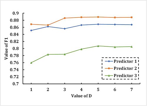
For PSSM_DT, selecting the appropriate dimension has a significant impact on the performance of iDRPro-SC. Low dimensional PSSM_DT cannot represent deep features of proteins, while high dimensional PSSM_DT consumes many computing resources, and parameter D determines the dimension of PSSM_DT. To select the appropriate parameter D, we conducted a 5-fold cross-validation experiment on the benchmark dataset to study the effect of parameter D on the performance of iDRPro-SC. The value of parameter D ranged from 1 to 7. As shown in Figure 3, we used F1 to evaluate the performance of the three base classifiers, including preditor 1, predictor 2 and predictor 3. With the increase of parameter D, the performance of the base classifier first improved and then mostly remained unchanged. When parameter D is 5, the performance is the best. Considering the prediction performance and calculation cost, we set the D of PSSM_DT to 5 in the following experiment. Table 2 shows the performance of three base classifiers in the 5-fold cross-validation experiment on the benchmark dataset when parameter D is set to 5. As shown in Table 2, the base classifiers achieved good performance.
The effect of parameter D on the three base classifiers in the 5-fold cross-validation experiment on the benchmark dataset.
The performance of base classifiers in the 5-fold cross-validation experiment on the benchmark dataset
| Class | ACC | MCC | SN | SP | PRE | F1 | Confidence interval of F1a |
|---|---|---|---|---|---|---|---|
| Predictor 1 | 0.86 | 0.71 | 0.88 | 0.83 | 0.85 | 0.87 | (0.862, 0.883) |
| Predictor 2 | 0.85 | 0.67 | 0.89 | 0.78 | 0.89 | 0.89 | (0.884, 0.896) |
| Predictor 3 | 0.85 | 0.69 | 0.84 | 0.86 | 0.77 | 0.81 | (0.809, 0.819) |
aThe confidence level is 95% at this location.
The combination of subfunction classifiers can improve the predictive performance
To study the effect of the subfunction predictor on the performance, we used the Basic-Model and iDRPro-SC to conduct a 5-fold cross-validation experiment on the benchmark dataset to evaluate their performance. Similar to iDRPro-SC, the Basic-Model uses PSSM_DT with parameter D set to 5, but the base classifiers are different. The Basic-Model does not combine subfunction classifiers in the base classifiers; that is, the base classifiers only include Predictors 1–3. We chose to integrate these three basic predictive factors into a basic model because they cover the most fundamental aspects of protein–nucleic acid interactions. By combining these three predictors, we can capture a wide range of NABP categories, including NABP classes with different binding specificities and structures. The detailed parameters of the Basic-Model can be found in Supplementary Information Table S1. Figure 4 and Table 3 show the performance of the Basic-Model and iDRPro-SC; the ACC, F1 and MCC of iDRPro-SC were better than those of the Basic-Model in the DBPs task and RBPs task, which further indicates that adding subfunction classifiers further improved the prediction of NABPs.
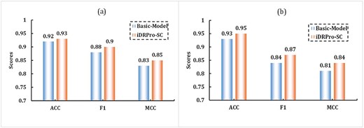
The performance comparison between the Basic-Model and iDRPro-SC in 5-fold cross-validation experiments on the benchmark dataset. (a) The performance comparison for DBPs task. (b) The performance comparison for RBPs task.
The performance comparison between the Basic-Model,iDRBP-ECHF and iDRPro-SC in 5-fold cross-validation experiments on the benchmark dataset
| Class | Method | ACC | MCC | F1 | Confidence interval of F1a |
|---|---|---|---|---|---|
| DNA-binding | Basic-Model | 0.92 | 0.83 | 0.88 | (0.877, 0.889) |
| iDRBP-ECHF | 0.94 | 0.86 | 0.91 | (0.909, 0.915) | |
| iDRPro-SC | 0.93 | 0.85 | 0.90 | (0.898, 0.909) | |
| RNA-binding | Basic-Model | 0.93 | 0.81 | 0.84 | (0.836, 0.845) |
| iDRBP-ECHF | 0.91 | 0.79 | 0.81 | (0.803, 0.813) | |
| iDRPro-SC | 0.95 | 0.84 | 0.87 | (0.868, 0.880) |
aThe confidence level is 95% at this location.
Comparison with existing methods on the TEST dataset TEST474
In this section, we compared the proposed method with several existing methods on the test dataset TEST474, including DNAbinder [8], RNAPred [13], StackDPPred [9], DPP-PseAAC [10], DeepDRBP-2L [17], IDRBP-PPCT [19], iDRBP-ECHF [18], DNAPred_Prot [32], DeepRBPPred [16], RBPPred [14], SPOT-Seq-RNA [11], catRAPID [12] and TriPepSVM [15]. To avoid overestimating the performance of iDRPro-SC on the test dataset TESE474, BLASTClust [23] was used to delete protein sequences in the benchmark dataset that had >25% redundancy with the test dataset. Finally, we reconstructed the benchmark dataset1, including 3918 RBPs, 7419 DBPs, 331 DRBPs and 10 062 NON-NABPs.
In the aforementioned methods, DeepDRBP-2L [17], IDRBP-PPCT [19] and iDRBP-ECHF [18] were retrained on the benchmark dataset to optimize the hyperparameters. However, the other methods cannot be retrained due to the corresponding source code being unavailable. Therefore, the results of the other methods were evaluated on the webserver. The results are shown in Table 4, from which we can show that the proposed method achieves better or comparable performance than the other state-of-the-art methods.
The performance comparison between iDRPro-SC and other methods on the Test Dataset TEST474
| Class | Method | ACC | REC | SP | PRE | F1 | MCC |
|---|---|---|---|---|---|---|---|
| DNA-binding | DNAbinder [6] | 0.75 | 0.89 | 0.66 | 0.62 | 0.73 | 0.54 |
| StackDPPred [7] | 0.68 | 0.89 | 0.55 | 0.56 | 0.68 | 0.44 | |
| DPP-PseAAC [8] | 0.75 | 0.89 | 0.66 | 0.62 | 0.73 | 0.54 | |
| DeepDRBP-2L [15] | 0.84 | 0.81 | 0.86 | 0.78 | 0.8 | 0.66 | |
| IDRBP-PPCT [17] | 0.89 | 0.83 | 0.93 | 0.88 | 0.85 | 0.77 | |
| iDRBP-ECHF [16] | 0.91 | 0.88 | 0.92 | 0.88 | 0.88 | 0.80 | |
| DNAPred_Prot [32] | 0.60 | 0.04 | 0.96 | 0.4 | 0.08 | −0.02 | |
| iDRPro-SC | 0.9 | 0.86 | 0.92 | 0.87 | 0.87 | 0.79 | |
| RNA-binding | RNAPred [11] | 0.48 | 0.82 | 0.42 | 0.21 | 0.34 | 0.18 |
| DeepRBPPred(balance) [14] | 0.36 | 0.8 | 0.28 | 0.17 | 0.29 | 0.07 | |
| DeepRBPPred(unbalance) [14] | 0.49 | 0.72 | 0.45 | 0.2 | 0.31 | 0.13 | |
| RBPPred [12] | 0.61 | 0.74 | 0.59 | 0.26 | 0.38 | 0.24 | |
| SPOT-Seq-RNA [9] | 0.8 | 0.11 | 0.94 | 0.26 | 0.15 | 0.07 | |
| catRAPID [10] | 0.53 | 0.41 | 0.56 | 0.15 | 0.22 | 0.03 | |
| TriPepSVM [13] | 0.86 | 0.54 | 0.92 | 0.55 | 0.55 | 0.46 | |
| DeepDRBP-2L [15] | 0.86 | 0.64 | 0.9 | 0.56 | 0.6 | 0.52 | |
| IDRBP-PPCT [17] | 0.89 | 0.63 | 0.94 | 0.66 | 0.64 | 0.58 | |
| iDRBP-ECHF [16] | 0.9 | 0.66 | 0.94 | 0.68 | 0.67 | 0.61 | |
| iDRPro-SC | 0.93 | 0.67 | 0.98 | 0.86 | 0.76 | 0.72 |
In this experiment, RBPs were regarded as negative samples in the DBPs task, while DBPs were regarded as negative samples in the RBPs task. The existing RBPs predictors incorrectly predicted a number of DBPs to be RBPs, and the existing DBPs predictors predicted a number of RBPs to be DBPs, resulting in lower F1. iDRPro-SC not only predicts DBPs and RBPs at the same time, but it also achieved a balanced performance in DBPs task and RBPs task. The ACC, F1 and MCC of iDRPro-SC were comparable to those of the existing DBPs/RBPs predictors. Therefore, the iDRPro-SC is suitable for the DBPs task and RBPs task.
Moreover, to evaluate the stability of the iDRPro-SC with the different redundancy thresholds between the test dataset and benchmark dataset, we utilized the BLASTCUT [23] to cutoff the sequences in the benchmark dataset that have >35% sequence similarity to any sequence in the test dataset TEST474. The reduced benchmark dataset2 included 7555 DBPs, 3927 RBPs, 3321 DRBPs and 10 131 NON-NABPs. Then the proposed method was retrained using the reduced benchmark dataset2 to predict the test dataset TEST474. The results of the proposed method on the test dataset TEST474 are shown in Table 5, from which we can show that the performance of the iDRPro-SC on the TEST474 test dataset is similar, demonstrating the stability of the proposed method.
The performance of the iDRPro-SC on the test dataset TEST474
| Class | Method | ACC | REC | SP | PRE | F1 | MCC |
|---|---|---|---|---|---|---|---|
| DNA-binding | iDRPro-SCa | 0.9 | 0.86 | 0.92 | 0.87 | 0.87 | 0.79 |
| iDRPro-SCb | 0.91 | 0.87 | 0.93 | 0.88 | 0.88 | 0.80 | |
| RNA-binding | iDRPro-SCa | 0.93 | 0.67 | 0.98 | 0.86 | 0.76 | 0.72 |
| iDRPro-SCb | 0.93 | 0.68 | 0.98 | 0.87 | 0.76 | 0.73 |
aDenotes the proposed method trained on the reduced benchmark dataset1
bDenotes the proposed method trained on the reduced benchmark dataset2
To further compare the comprehensive performance of the predictor, we used Ranking_Score to compare the comprehensive performance of the predictor on the DBPs task and RBPs task. The Ranking_Score is the sum of the DBP_Rank and RBP_Rank, and a smaller Ranking_Score indicates better prediction performance. As shown in Table 6, iDRPro-SC and iDRBP-ECHF achieved the best performance, and the iDRPro-SC model is lighter. These results show that the iDRPro-SC proposed in this study is superior to other methods and can capture the features of different types of NABPs, enabling better distinction among them.
The comparison of Ranking_Score of different methods on the test dataset
| Method | DBP_F1 | DBP_Rank | RBP_F1 | RBP_Rank | Ranking_Score |
|---|---|---|---|---|---|
| iDRPro-SC | 0.87 | 2 | 0.76 | 1 | 3 |
| iDRBP-ECHF | 0.88 | 1 | 0.67 | 2 | 3 |
| IDRBP-PPCT | 0.85 | 3 | 0.64 | 3 | 6 |
| DeepDRBP-2L | 0.8 | 4 | 0.6 | 4 | 8 |
| Method | DBP_F1 | DBP_Rank | RBP_F1 | RBP_Rank | Ranking_Score |
|---|---|---|---|---|---|
| iDRPro-SC | 0.87 | 2 | 0.76 | 1 | 3 |
| iDRBP-ECHF | 0.88 | 1 | 0.67 | 2 | 3 |
| IDRBP-PPCT | 0.85 | 3 | 0.64 | 3 | 6 |
| DeepDRBP-2L | 0.8 | 4 | 0.6 | 4 | 8 |
Comparsion with the StackDPPred method on the test datasets PDB186 and PDB676
In this section, we evaluate the performance of iDRPro-SC on the two test dataset, including PDB186 [9] and PDB676 [9]. To avoid overestimating the performance of the proposed method, for each target test dataset, the sequences in the benchmark dataset sharing >25% similarities with any sequences in the corresponding test dataset are removed. Therefore, we constructed the corresponding benchmark dataset related to the different test datasets to optimize the parameters. For the PDB186 test dataset, the corresponding benchmark dataset contains 7552 DBPs, 3939 RBPs, 332 DRBPs and 10 155 NON-NABPs. For the PDB676 test dataset, the corresponding benchmark dataset contains 7399 DBPs, 3931 RBPs, 330 DRBPs and 10 016 NON-NABPs.
The results are shown in Table 7, from which we can see that the proposed method achieves similar performance to StackDPPred [9]. StackDPPred utilizes four properties features to encode the proteins, including PSSM, RCEM, PSSM-DT and RPT. The RCEM features are constructed based on the 3D structural information from the PDB. However, the proposed method merely utilizes the PSSM feature encoding. Several sequences in the benchmark dataset cannot obtain the corresponding 3D structural information from PDB files. Therefore, the iDRPro-SC is a useful tool for DBPs prediction.
Feature analysis
To examine why iDRPro-SC outperforms the Basic-Model, we further compared the ensemble feature distributions of the two models on the test dataset. We used UMAP [43] to map the ensemble features of these two models into two-dimensional space to visualize their feature distribution. As shown in Figure 5, the ensemble features of iDRPro-SC more easily distinguish different types of proteins than the ensemble features of the Basic-Model. For this reason, iDRPro-SC has better performance than the Basic-Model, which further verifies that the subfunction predictors can improve the performance of NABPs predictors.
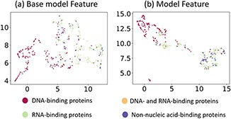
Visualization of the ensemble features generated by Basic-Model and iDRPro-SC on test dataset TEST474. (a) The ensemble feature of the Basic-Model. (b) The ensemble feature of the iDRPro-SC.
Application of iDRPro-SC to Tomato genome annotation on ITAG4.1
NABPs predictors can annotate DBPs and RBPs by using protein sequence information. To study the wide applicability of iDRPro-SC, we used it to annotate the tomato genome using the tomato genome dataset (ITAG4.1) [44]. Previous studies have shown that DBPs account for 6–8% of the proteome in eukaryotes, while RBPs account for 6–7% [7]. The ITAG4.1 dataset contains 34 075 protein sequences, which were annotated according to the information in the UniProtKB database. In this experiment, we selected 2100 prediction DBPs and 2100 prediction RBPs using the prediction scores and counted the prediction results in accordance with the keywords in UniProtKB. Figure 6 shows the percentage of correct DBPs\RBPs predicted by different methods among all DBPs\RBPs. The prediction results of iDRPro-SC included more proteins annotated by DBPs\RBPs in UniProtKB, which indicates that our method is superior to other methods in identifying NABPs in the tomato genome annotation and has good applicability.
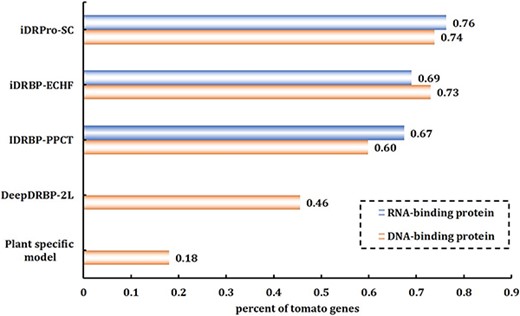
The performance comparison of different methods for predicting DBPs and RBPs on ITAG4.1.
CONCLUSION
In this paper, we propose a new method called iDRPro-SC to predict DBPs and RBPs that integrates the subfunction of the protein, thereby further improving the prediction performance. iDRPro-SC uses evolutionary information PSSM to extract protein features, bi-LSTM to construct base classifiers and RF to construct classifiers to identify DBPs and RBPs. The performance comparison between iDRPro-SC and other methods on the test dataset showed that iDRPro-SC was superior to other methods, indicating that it has good prediction performance. The results of ITAG4.1 experiment showed the applicability of iDRPro-SC in real-world scenarios. The results of the feature analysis showed that iDRPro-SC combined with the subfunction classifiers can better extract its features, so that it more easily distinguishes different kinds of proteins. We have also developed a web server for iDRPro-SC that can be accessed at http://bliulab.net/iDRPro-SC. This will be a useful tool to identify DBPs and RBPs. iDRPro-SC provides a new perspective for the problems in the field of bioinformatics. In the future, the ensemble learning framework has many potential fields, such as anti-cancer peptide prediction [29], peptide function recognition [3], etc.
iDRPro-SC considers the internal differences of NABPsand combines their subfunctions to identify DNA- and RNA-binding proteins.
Experimental results on the datasets showed that iDRPro-SC outperforms the other competing methods. The results of ITAG4.1 experiment showed the applicability of iDRPro-SC in real-world scenarios.
We developed the corresponding web server of iDRPro-SC, which can be accessed at http://bliulab.net/iDRPro-SC, and it would be a useful tool for identifying DNA- and RNA-binding proteins.
ACKNOWLEDGEMENTS
We are very indebted to the three anonymous reviewers, whose constructive comments have been very helpful in strengthening the paper. We thank Gabrielle White Wolf, PhD, from Liwen Bianji (Edanz) (www.liwenbianji.cn) for improving the English text of a draft of this manuscript.
FUNDING
This work was supported by the National Natural Science Foundation of China (No. 62102030,62271049 and U22A2039) and National Key R&D Program of China (No. 2022YFC3302101).
Author Biographies
Ke Yan is currently an Assistant Professor with the School of Computer Science and Technology, Beijing Institute of Technology University, Beijing, China. His research interests include bioinformatics, pattern recognition and machine learning.
Jiawei Feng is a master student at the School of Computer Science and Technology, Beijing Institute of Technology, China. His expertise is in bioinformatics.
Jing Huang is an Associate Researcher at Huajian Yutong Technology (Beijing) Co., Ltd; State Key Laboratory of Media Convergence Production Technology and Systems, Beijing, China, 100803; Xinhua New Media Culture Communication Co., Ltd. Her expertise is in nature language processing.
Hao Wu, PhD, is an experimentalist at the School of Computer Science and Technology, Beijing Institute of Technology, Beijing, China. His expertise is in bioinformatics, nature language processing and machine learning.
REFERENCES
Dixit S.
Author notes
Ke Yan and Jiawei Feng contributed equally to this work.
