


Abstract
As the volume of protein sequence and structure data grows rapidly, the functions of the overwhelming majority of proteins cannot be experimentally determined. Automated annotation of protein function at a large scale is becoming increasingly important. Existing computational prediction methods are typically based on expanding the relatively small number of experimentally determined functions to large collections of proteins with various clues, including sequence homology, protein–protein interaction, gene co-expression, etc. Although there has been some progress in protein function prediction in recent years, the development of accurate and reliable solutions still has a long way to go. Here we exploit AlphaFold predicted three-dimensional structural information, together with other non-structural clues, to develop a large-scale approach termed PredGO to annotate Gene Ontology (GO) functions for proteins. We use a pre-trained language model, geometric vector perceptrons and attention mechanisms to extract heterogeneous features of proteins and fuse these features for function prediction. The computational results demonstrate that the proposed method outperforms other state-of-the-art approaches for predicting GO functions of proteins in terms of both coverage and accuracy. The improvement of coverage is because the number of structures predicted by AlphaFold is greatly increased, and on the other hand, PredGO can extensively use non-structural information for functional prediction. Moreover, we show that over 205 000 (|$\sim $|100%) entries in UniProt for human are annotated by PredGO, over 186 000 (|$\sim $|90%) of which are based on predicted structure. The webserver and database are available at http://predgo.denglab.org/.
INTRODUCTION
Recent advances in genome sequencing and structural genomics are increasing the abundance of experimental sequences and three-dimensional structures, which need functional characterization. The gap between the large number of proteins that have been identified and the completeness of their annotations is continually widening. For example, as of November 2022, nearly 484 700 (|$\sim $|85%) protein sequences deposited into the UniProtKB/Swiss-Prot database were without manually curated function; the same is true for many structures in the Protein Data Bank (PDB), nearly 156 300 (|$\sim $|74%) structures lacked manually assigned function, and even after putative automated annotations nearly 111 900 (|$\sim $|53%) structures remain listed as unannotated in the Gene Ontology Annotation (GOA) database [1]. Experimental identification and manual protein function annotation remain labor-intensive and expensive tasks. Consequently, in this scenario, researchers have focused on developing accurate computational methods for protein function prediction, which can therefore aid in reducing the gap.
With the ever-increasing accumulation of sequence and structure information, coupled with massive high-throughput experimentally data, a number of computational methods have been proposed to exploit these heterogeneous data, including function prediction from the amino acid sequence [2–4], structure data [5], gene expression [6], protein–protein interaction [7, 8], genomic context [9] and integrated methods [10–16].
The most common approach for protein function prediction is to use homology or sequence similarity and transfer functional annotations to newly identified proteins. Global and local sequence alignments, such as FASTA [17], BLAST and PSI-BLAST [18], are used to query sequence databases for homologs with a target protein, and the known functions of the top hits are transferred to the query. A better strategy for homology-based functional annotation is PFP [3], which uses three rounds of PSI-BLAST and a so-called ’function association matrix’ to include the annotations of even remote homologs. The extended similarity group (ESG) method [4], which performs iterative sequence database searches, promises to be more sensitive and accurate than conventional PSI-BLAST and its predecessor PFP. In recent years, a series of deep-learning methods have been proposed. These methods usually extract sequence features by calculating sequence similarity, multiple sequence alignments and sequence motifs and use neural networks to build the prediction model [19–24]. In addition to this, sequence-based protein language models have also yielded very promising results in protein bioinformatics and even in the whole protein science [25–28]. Although the sequence-based transfer is a genuine way of inferring function in the light of evolution, practically, a precise function is conserved only at levels of sequence identity >40% [29] and most of the newly identified proteins do not show significant sequence similarity with experimentally annotated proteins. Additionally, sequence similarity does not always imply functional equivalence; thus, sequence-based functional transfers can be erroneous. For example, proteins from gene duplication may have high sequence similarity but a divergence of functions. In addition, misannotations can be spread even when homology-based approaches are used in manually curated databases.
When sequence-based methods fail, functional clues can be inferred from the protein’s three-dimensional structure since the protein’s structure often remains more conserved than its sequence [30]. Methods for predicting function from structure rely on detecting some structural similarity, whether global or local, between the target protein and a structure of the known function. Global structure-comparison algorithms (e.g. DALI [31], TM-align [32] and MADOKA [33]) can be used to exploit general structural similarity. Other methods identify local surface regions that may be associated with highly specific functions. Examples include pvSOAR [34], eF-site [35], PDBSiteScan [36] and so on. However, structural information has not been widely used for protein function annotation. One of the main reasons is that there is a significant gap between the number of proteins with known sequences and those with experimentally determined structures. Recently, AlphaFold2 [37] has made a major breakthrough in the protein folding problem by predicting the 3D structure of proteins with atomic-level precision based on amino acid sequences alone [38]. And the model trained only on virtual samples predicted by AlphaFold2 is able to perform comparably to models based on experimentally solved real structures. These provide favorable conditions for improving the performance of structure-based protein function prediction.
In this paper, we propose a computational protein function prediction approach termed PredGO, which achieves high-performance protein function prediction by using a protein language model ESM-1b [39] trained by a large number of protein sequences to extract sequence features, graph neural network with geometric vector perceptron (GVP–GNN) [40] to extract protein structures predicted by AlphaFold2 and the multi-head attention mechanism to fuse protein-protein interaction (PPI) features. It can be observed from the comparison experiments that our model is able to extract the information in the predicted protein structures and achieve high-performance prediction of protein functions even if only sequence information is available. In addition, we experimentally verify the performance of the model for specific species. And we observe the difference between our model and competing methods in prediction results through specific proteins. We finally apply PredGO to human genome-wide protein function prediction and obtain promising results.
MATERIALS AND METHODS
Datasets
We used two datasets, CAFA3 [41–43] and UniGOA16, to evaluate methods. We downloaded the CAFA3 dataset from DeepGOPlus (https://deepgo.cbrc.kaust.edu.sa/data/) [23]. This dataset includes the CAFA3 challenge training sequences and experimental annotations released in September 2016, as well as the test benchmarks released on November 15, 2017. We removed proteins with sequence lengths greater than 1000 and proteins with ’fuzzy’ amino acids, such as consortia or unknowns. After processing, there are 3039 proteins in the test set. We obtained the protein structures from AlphaFoldDB (https://alphafold.ebi.ac.uk/download) [44]. For proteins in the test set whose structures could not be downloaded from AlphaFoldDB, we used the local version of AlphaFold2 to make predictions with the preset of ’full_dbs.’ We extracted the PPI information from the STRING database [45]. We filtered the PPI using medium confidence (|$\geq $|0.4). To ensure the fairness of the evaluation, we downloaded the STRING database version 10.0 (http://version10.string-db.org/), released on April 16, 2016, before the release time of the CAFA3 training set.
We also built a dataset termed UniGOA16 from the UniProt-GOA [1] according to the standard CAFA protocol. We used the same GO version and STRING database as the CAFA3 dataset. We downloaded protein sequences from UniProt (https://www.uniprot.org/downloads) [46], predicted protein structures from AlphaFoldDB and protein functional annotations from GOA (http://www.ebi.ac.uk/GOA). We extracted all experimental annotations and removed unpredictable proteins and GO terms. We used the proteins experimentally annotated before June 24, 2016 as the training set, the no-knowledge proteins experimentally annotated from June 24, 2016 to June 24, 2019 as the validation set, and the no-knowledge proteins experimentally annotated from June 24, 2019 to January 1, 2022 as the test set. Finally, we used MMseqs2 [47] to cluster all sequences in the dataset with 60% sequence identity, removing sequences in the validation and test sets that appear in the same cluster as the training set sequences. Table 1 shows the statistics for both datasets.
Summary of the CAFA3 and UniGOA16 datasets
| Dataset | Ontology | Training | Validation | Test | Terms |
|---|---|---|---|---|---|
| CAFA3 | MFO | 28 679 | 3228 | 1035 | 677 |
| BPO | 42 250 | 4748 | 2185 | 3992 | |
| CCO | 39 893 | 4510 | 1117 | 551 | |
| UniGOA16 | MFO | 38 585 | 1315 | 1058 | 613 |
| BPO | 53 056 | 2068 | 1305 | 3531 | |
| CCO | 49 605 | 2506 | 1956 | 534 |
PredGO
Overview
As illustrated in Figure 1, PredGO comprises five key steps: data search and generation, protein sequence feature extraction, PPI feature fusion, structure feature extraction, feature concatenation and GO term prediction.
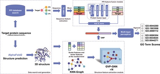
An overview of PredGO. The input is a protein sequence. PredGO first searches for interacting proteins from the STRING database and predicts the protein structure using AlphaFold2. Then the protein sequence features are extracted by ESM-1b, and the proteins with interactions are fused using a PPI feature fusion module with protein fusion layers. The predicted structures are represented in the structure feature extraction module as graph structures with scalar features and vector features and extracted by GVP-GNN. Finally, the sequence-based and PPI-based features are concatenated with structure-based features to obtain the scores of GO terms by a multilayer perceptron and sigmoid function.
The data search and generation step serves two main purposes. Firstly, it utilizes AlphaFold2 to generate 3D structural data for proteins. Secondly, it searches the database to retrieve other proteins that interact with the target protein. This step provides crucial inputs for the subsequent feature extraction process.
The sequence feature extraction module, PPI feature fusion module and structure feature extraction module are responsible for extracting relevant features from the obtained data. These modules play an essential role in capturing important characteristics of proteins.
Finally, the feature concatenation and term prediction steps integrate the extracted features to predict protein functions based on GO terms.
Protein sequence feature extraction
The protein language model ESM-1b, pre-trained using massive data, can effectively represent protein sequences as a vector. For a protein sequence of length |$n$|, the output of this model is a vector |$p \in \mathbb{R}^{n \times 1280}$|. We average the first dimension of the vector |${p=(a_1,a_2,...,a_n)^{\mathrm{T}}}$| to get a new vector |$p^{\prime} \in \mathbb{R}^{1280}$| of fixed length, and use this vector to represent the protein.
Assuming that there are |$m$| proteins that can be searched from the PPI database that have interactions with the target protein |$t$|, then there will be |$m+1$| protein sequences to be input into the model. After the above processing, a vector |$H^E_t = (p^{\prime}_0,p^{\prime}_1,p^{\prime}_2,...,p^{\prime}_m)^{\mathrm{T}} \in \mathbb{R}^{ (m+1) \times 1280}$| will be obtained, where |$p^{\prime}_0$| represents the vector of the target protein, and the other is the vector of the interacting proteins.
PPI feature fusion module
Referring to the Encoder module in the Transformer model [48], we designed the PPI feature fusion module. This module consists of multiple protein fusion layers that can be stacked and a residual connection layer.
The protein fusion layer consists of multi-headed attention mechanisms and feed-forward neural networks. It treats proteins with interactions as different words in a sentence, and each protein is able to fuse useful information from other proteins using the multi-headed attention mechanism. In the multi-headed attention mechanism, the vectors of each protein will be linearly transformed to generate multiple sets of vectors |${Q}$|, vectors |${K}$| and vectors |${V}$|, where |${Q}$| and |${K}$| are used to determine the weights of protein fusions, and |${V}$| is the value being fused. After the multi-attention mechanism layer and feedforward neural network, we use residual connection [49], droupout [50] and layer normalization [51] to avoid the occurrence of gradient disappearance and overfitting. To avoid interacting proteins losing their original information when features are fused, we merge the unprocessed vector with the processed vector using the residual connection to obtain the final feature. This feature contains the sequence information and PPI information of the protein. The multiheaded attention mechanism and feed-forward neural network can be calculated as follows:
Where |$head_i=Attention(H^E_tW^Q_i,H^E_tW^K_i,H^E_tW^V_i)$|.
where |$W^Q_i \in \mathbb{R}^{d_{model} \times d_k}$|, |$W^K_i \in \mathbb{R}^{d_{model} \times d_k}$|, |$W^V_i \in \mathbb{R}^{d_{model} \times d_v}$|, |$W^o \in \mathbb{R}^{hd_v \times d_{model}}$|, |$W_1 \in \mathbb{R}^{d_{model} \times 4d_{model}}$|, |$W_2 \in \mathbb{R}^{4d_{model} \times d_{model}}$| are the parameter matrices of the projection. |$h$| is the number of heads, |$d_k=d_v=d_{model}/h=1280/h$|, |$b_1$| and |$b_2$| are the bias terms.
Taking the vector |$H^E_t$| input to protein fusion layers as an example, a new vector |${H^{E}_t}^{\prime}= (p_0^{\prime\prime},p_1^{\prime\prime},p_2^{\prime\prime},...,p_m^{\prime\prime})^{\mathrm{T}} \in \mathbb{R}^{(m+1) \times 1280}$| will be obtained after processing by the protein fusion layers. After further processing by residual concatenation |$v_{sp}=LayerNorm(dropout(p^{\prime}_0+p^{\prime\prime}_0))$|, a vector |$v_{sp}\in \mathbb{R}^{1280}$| containing sequence information and PPI information will be obtained to represent the target protein.
Structure feature extraction module
We use GVP–GNN [40] to extract the information contained in the 3D structure. GVP can be viewed as an extension of linear transformation that can compute both scalar and vectors. All nodes and edges in this GNN are represented using tuples containing scalars and vectors, enabling efficient representation of 3D structures of large biomolecules, including protein, through geometric and relational reasoning. GVP takes a pair of scalar features |$s \in \mathbb{R}^{n}$| and vector features |$V \in \mathbb{R}^{3 \times v}$| as input and outputs new scalar features |$s^{\prime} \in \mathbb{R}^{m}$| and vector features |$V^{\prime} \in \mathbb{R}^{3 \times \mu }$|. The calculation process is as follows:
where |$V_h = VW_h$|. |$W_h \in \mathbb{R}^{v \times h}$|, |$W_m \in \mathbb{R}^{(n+h) \times m} $| and |$W_\mu \in \mathbb{R}^{h \times \mu } $| are the parameter matrices of the projection, b is the bias term, and |$\sigma $| and |$\sigma ^+$| are the activation functions.
GVP–GNN uses the message passing mechanism [52] to update node embeddings with messages from adjacent nodes and edges. Assume that |$h^{(j)}_v$| and |$h^{(j\rightarrow i)}_e$| represent the embedding of node j and edge (|$\,j\rightarrow i$|), the message passed from node |$j$| to node |$i$| can be expressed as |$h^{(j\rightarrow i)}_m = g(Concat(h^{(j)}_v,h^{(j\rightarrow i)}_e)) $|, where |$g$| represents a function with GVPs. The steps of graph propagation are as follows:
where |$k^{\prime}$| is the number of incoming messages. Between graph propagation steps, the network uses GVP to update the node embeddings including scalar features and vector features at all nodes. The update process is as follows:
In this module, we create a KNN-graph by connecting adjacent nodes based on the |$C\alpha $| atom coordinates. Then, we construct scalar and vector features for both nodes and edges.
For instance, consider the |$ith$| node, where the |$C_i$| atom represents the |$ith$| node’s C atom. The node’s scalar features comprise the sine and cosine values of dihedral angles. These angles are computed using |$N_i$|, |$C\alpha _i$|, |$C_i$|, |$C_{i-1}$| and |$N_{i+1}$|. On the other hand, the vector feature of the node consists of forward and reverse unit vectors in the direction of |$C\alpha _{i+1}-C\alpha _i$| and |$C\alpha _{i-1}-C\alpha _i$|, respectively. We also estimate the unit vectors in the direction of |$C\beta _{i}-C\alpha _i$| by assuming tetrahedral geometry and normalization [40].
To encode edges, we utilize the Gaussian radial basis functions and sine encoding with relative position information [48] for the scalar feature. In contrast, the vector feature of the edge represents the direction formed by the |$C\alpha $| atoms at its ends.
For a protein containing |$n$| residues, after being processed by the structure feature extraction module, a vector |$v_s \in \mathbb{R}^{n \times d_s}$| will be obtained, where the first dimension is the feature representation of each residue,|$d_s$| is the dimension of each residue node output by GVP–GNN.
Feature concatenation and term prediction
We combine the output of the PPI feature fusion module and the structure feature extraction module for GO term prediction. Since the vector |$v_s$| output from the structure feature extraction module is at the residue level, it first needs to be converted into a protein-level vector |$v_s^{\prime} \in \mathbb{R}^{d_s}$| using the global mean pooling layer (GMP). Then, |$v_s^{\prime}$| is concatenated with the vector |$v_{sp}$| from the PPI feature extraction module to obtain the final representation vector |$v_{target}$| of the target protein. Next, the dimensionality of this embedding is transformed into the dimensionality of the number of GO terms using a multilayer perceptron (MLP). Finally, the predictions of the model are transformed into confidence scores |$s_p$| from 0 to 1 using a sigmoid function. The calculation process is as follows:
Training
We implemented the model in Pytorch and Pytorch Geometric library [53, 54], and trained our model with binary cross-entropy as loss function and AdamW optimizer [55] with a learning rate of 1E-3. We set the dropout rate to 0.2 and use two layers of GVP–GNN, two protein fusion layers and three-layer multilayer perceptron, where the dimension of MLP layer 1 is the sum of the output feature dimension of the structure feature extraction module and the PPI feature fusion module, the dimension of layer 2 is four times that of layer 1, and the dimension of layer 3 is the number of predicted GO terms. We trained six models on the CAFA3 and UniGOA16 datasets for Molecular Function Ontology (MFO), Biological Process Ontology (BPO) and Cellular Component Ontology (CCO), respectively. During the training period, the model with the highest |$F_{max}$| value on the validation set is retained as the final model. The CAFA3 dataset’s epoch and batch sizes of training MFO, BPO and CCO models are 15, 20, 15 and 24, 24, 36. And on the UniGOA16 dataset, the epoch and batch sizes of training MFO, BPO and CCO models are 10, 15, 10 and 36, 36, 24.
Competing methods
Naive approach
Due to the hierarchical structure of GO terms, more annotations are generated in high-level GO terms. Predictions are obtained by simply calculating the GO term frequencies in the training set and assigning them across all proteins. This method, called ’naive’ in CAFA, is used as a baseline for comparing methods [43]. The calculation method is as follows:
where |$p_i$| is the target protein, |$G_j$| is the GO term to be predicted, |$N_j$| is the number of occurrences of |$G_j$| in the training set and |$N_{total}$| is the number of proteins in the training set.
DiamondBLAST and DiamondScore
Proteins with similar sequence tend to have similar functions. A basic approach to function prediction is to use BLAST to find proteins with similar sequence in the training set, assigning functions of similar proteins to target proteins [18]. We use Diamond to find similar sequence in the training set, and get a set of bitscores about query sequence and similar sequence [56]. We use the maximum normalized bitscore from similar sequence as the predicted value of the target protein |$p_{i}$|:
where |$S(p_i)$| represents a set of proteins with similar sequence to protein |$p_i$| filtered by e-value of 0. 001, |$T(G_j,p_s)$| returns 1 if |$G_j$| is a true annotation of protein |$p_s$| and 0 otherwise. The |$bitscore$| is the similarity score of the protein |$p_i$| and |$s$| calculated by Diamond.
DiamondBLAST considers only the most similar sequences, while DiamondScore uses all the similar sequences returned by Diamond to predict the function. The calculation method is as follows:
DeepGOCNN and DeepGOPlus
DeepGOCNN and DeepGOPlus are well-known deep learning methods that predict only from sequence. DeepGOCNN uses a 1D CNN to scan protein sequences and uses a flat classification layer as a classifier to predict protein functions [23]. It can predict protein functions efficiently and in a wide range. DeepGOPlus combines the output of DeepGOCNN with the output of DiamondScore to further improve the prediction performance. We downloaded the source code of these methods, and according to the description in the paper, we selected different sizes of CNN filters for training on the training set, and selected the model with the best performance on the validation set as the final result, and finally selected the filters of sizes {8, 16, 24,..., 128}. For DeepGOPlus, we selected the alpha parameter that performed best on the validation set for combining DiamondScore.
LR-ESM
Large-scale protein language models have achieved surprising performance in protein-related fields. Esm-1b is a state-of-the-art protein language model that can be used to predict structure, function and other protein properties directly from individual sequence [39]. We convert the residue-level embedding of the model output to protein-level embedding by averaging the features at each residue level, and then use logistic regression (LR) to predict GO terms.
Evaluation metrics
We used three evaluation metrics to measure the performance of the method: |$F_{max}$|, |$S_{min}$| and area under the precision–recall curve (AUPR). |$F_{max}$| and |$S_{min}$| are used as the main evaluation metrics in CAFA [41, 43]. AUPR is widely used in the evaluation of multi-label classification tasks including protein function prediction [57, 58]. |$F_{max}$| is a protein-centeric evaluation metric, which is defined as follows:
where |$t$| is a prediction threshold with a step size of 0.01 between 0 and 1. |$k(t)$| is the number of proteins with at least one GO term score not less than |$t$|. |$n$| is the total number of proteins. |$1(\cdot )$| is 1 if the input is true, otherwise 0.
|$S_{min}$| is a term-centric evaluation metric that calculates the semantic distance between true annotations and predicted annotations. It is calculated as follows:
where |$ru(t)$| is called remaining uncertainty and |$mi(t)$| is called misinformation. |$IC(G_j)$| is the information content of term |$G_j$|. The function |$Pr$| represents the conditional probability. |$Parent(G_j)$| denotes the parent node of |$G_j$| in the GO hierarchy.
RESULTS
To evaluate the performance of our model, we conducted several different experiments. Among them, the ’Performance comparison of different feature combinations’ was carried out using the UniGOA16 dataset. The datasets for the experiments titled ’Performance on proteins with and without PPI information’ and ’Performance comparison on different species’ were obtained by segmenting the UniGOA16 dataset. The specific statistics are shown in Table 2.
Statistics on the number of sub-datasets used in the experiment
| Sub-dataset | MFO | BPO | CCO |
|---|---|---|---|
| UniGOA16 | 1058 | 1305 | 1956 |
| Proteins with PPI | 953 | 1081 | 1740 |
| Proteins without PPI | 104 | 224 | 216 |
| Human proteins | 145 | 119 | 163 |
| Mouse proteins | 64 | 124 | 109 |
| Fission yeast proteins | 11 | 25 | 20 |
| Sub-dataset | MFO | BPO | CCO |
|---|---|---|---|
| UniGOA16 | 1058 | 1305 | 1956 |
| Proteins with PPI | 953 | 1081 | 1740 |
| Proteins without PPI | 104 | 224 | 216 |
| Human proteins | 145 | 119 | 163 |
| Mouse proteins | 64 | 124 | 109 |
| Fission yeast proteins | 11 | 25 | 20 |
Performance on the test data set
As shown in Table 3, PredGO performs best in all three ontology domains for both datasets. On the CAFA3 dataset, PredGO has |$F_{max}$| of 0.674, 0.585, 0.699, |$S_{min}$| of 6.194, 18.067, 6.717 and AUPR of 0.642, 0.512, 0.678, respectively. On the UniGOA16 dataset, the |$F_{max}$| of PredGO was 0.687, 0.405, 0.694, the |$S_{min}$| was 3.719, 17.947, 5.442, and the AUPR was 0.603, 0.312, 0.734, respectively. The differences in performance between the different ontologies on the two datasets are caused by the structure and complexity of the ontologies and the available annotations. We can draw the following conclusions by comparing the results in the Table:
Performance comparison on the CAFA3 and UniGOA16 datasets
| Method | |$\boldsymbol{F_{max}}$| | |$\boldsymbol{S_{min}}$| | AUPR | ||||||
|---|---|---|---|---|---|---|---|---|---|
| MFO | BPO | CCO | MFO | BPO | CCO | MFO | BPO | CCO | |
| CAFA3 | |||||||||
| Naive | 0.444 | 0.406 | 0.613 | 8.989 | 21.859 | 7.872 | 0.328 | 0.285 | 0.572 |
| DiamondBLAST | 0.549 | 0.483 | 0.600 | 9.186 | 29.500 | 9.108 | 0.302 | 0.217 | 0.354 |
| DiamondScore | 0.610 | 0.529 | 0.436 | 6.723 | 19.464 | 7.354 | 0.634 | 0.322 | 0.473 |
| DeepGOCNN | 0.499 | 0.401 | 0.645 | 8.380 | 21.212 | 7.540 | 0.436 | 0.321 | 0.570 |
| DeepGOPlus | 0.599 | 0.520 | 0.664 | 7.605 | 20.117 | 7.345 | 0.507 | 0.368 | 0.587 |
| LR-ESM | 0.649 | 0.556 | 0.682 | 6.483 | 19.081 | 6.951 | 0.631 | 0.455 | 0.670 |
| PredGO | 0.674 | 0.585 | 0.699 | 6.194 | 18.067 | 6.717 | 0.642 | 0.512 | 0.678 |
| UniGOA16 | |||||||||
| Naive | 0.452 | 0.304 | 0.638 | 5.335 | 19.946 | 6.674 | 0.288 | 0.184 | 0.595 |
| DiamondBLAST | 0.507 | 0.318 | 0.475 | 5.903 | 26.360 | 7.506 | 0.273 | 0.090 | 0.269 |
| DiamondScore | 0.556 | 0.360 | 0.510 | 4.054 | 18.620 | 6.629 | 0.400 | 0.146 | 0.349 |
| DeepGOCNN | 0.528 | 0.329 | 0.646 | 5.185 | 19.735 | 6.553 | 0.362 | 0.193 | 0.603 |
| DeepGOPlus | 0.576 | 0.378 | 0.637 | 4.597 | 19.352 | 6.485 | 0.443 | 0.192 | 0.589 |
| LR-ESM | 0.660 | 0.385 | 0.680 | 4.031 | 18.400 | 5.706 | 0.572 | 0.292 | 0.705 |
| PredGO | 0.687 | 0.405 | 0.694 | 3.719 | 17.947 | 5.442 | 0.603 | 0.312 | 0.734 |
Note: Best performance in bold.
(i) On both datasets, compared with LR-ESM, PredGO improved |$F_{max}$| by 4.0%, 5.2% and 2.3%, decreased |$S_{min}$| by 6.1%, 3.9% and 4.0%, and improved AUPR by 3.5%, 9.7% and 2.7% on average for MFO, BPO and CCO. It can be seen that combining more information can improve the model performance compared to just using the protein language model.
(ii) DeepGOCNN uses only sequence information from the training set. PredGO and LR-ESM use protein language models pre-trained with a large amount of protein sequence data. From the average results of both datasets, PredGO improved |$F_{max}$| by about 32.6%, 34.5% and 7.90%, decreased |$S_{min}$| by 27.2%, 11.9% and 13.9%, and improved AUPR by 56.9%, 60.6% and 20.3% on MFO, BPO and CCO. From the experimental results, it is clear that pre-trained language models with a large number of sequences can effectively improve model performance.
(iii) The traditional methods based on sequence similarity, DiamondBLAST, and DiamondScore, outperformed the naive method in MFO and BPO but performed poorly in CCO. DeepGOPlus combining DeepGOCNN and DiamondScore improved the |$F_{max}$| of MFO and BPO by more than 9.1% on both datasets but decreased the |$F_{max}$| of CCO by 1.3% on the UniGOA16 dataset. This may be related to the fact that sequence homology carries more information related to molecular functions and biological processes and less information related to cellular components. PredGO improves by at least about 3.6%, and at most, can improve about 61.7% in each metric compared to the above methods. It shows that deep learning models are able to learn deeper information than sequence homology from a large number of sequences or other features for functional prediction.
Comparison with CAFA3 methods
We utilized the official CAFA evaluation tool to assess the performance of our model, trained on the CAFA3 dataset [41, 43]. It is important to note that the number of proteins in our training set is smaller than the number of proteins in the provided CAFA3 training dataset (|$\sim $|88%). We achieved this reduction by excluding proteins with lengths exceeding 1000 and those containing ’fuzzy’ amino acids, for which structure and sequence information extraction was challenging. To ensure comprehensive predictions on the benchmark data, we discarded the parts that required structural information in cases where structure prediction was not feasible.
The evaluation results are displayed in Figure 2. Notably, our model, PredGO, attained |$F_{max}$| scores of 0.56, 0.38 and 0.65 in the BPO, MFO and CCO evaluations, respectively. It ranked first in the CCO evaluation, second in the MFO evaluation and third in the BPO evaluation. These rankings exhibit slight differences compared to our internal evaluation results. These variations can be attributed to the fact that our model is primarily trained on proteins with lengths below 1000. Consequently, when the length exceeds this threshold, the predicted structure may be significantly affected by sequence truncation, leading to the loss of critical information and negatively impacting the model’s performance.
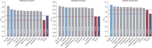
Comparison of PredGO with CAFA3 top 10 methods.
Moreover, it is noteworthy that the top-ranked method in the MFO and BPO evaluations is Zhu lab’s method, which integrates multiple classifier components using an ensemble learning approach, while the second-ranked method in the BPO evaluation is INGA-Tosatto, which employs a more diverse set of features [21, 59]. In contrast, PredGO is a model that can be integrated as a component in Zhu lab’s method and does not utilize ’dark’ proteomic information. This distinction may contribute to PredGO not being the best-performing model in the MFO and BPO evaluations.
Performance on proteins with and without PPI information
PredGO searches the database for PPI information, but not all proteins yield results, especially some newly discovered proteins for which there is rather little relevant information. To measure the performance of the model when only sequence information is available, we divided the test set of UniGOA16 according to whether PPI information can be searched from the database. Performance of PredGO versus competing methods is shown in Table 4.
Performance on proteins with and without PPI information
| Method | |$\boldsymbol{F_{max}}$| | |$\boldsymbol{S_{min}}$| | AUPR | ||||||
|---|---|---|---|---|---|---|---|---|---|
| MFO | BPO | CCO | MFO | BPO | CCO | MFO | BPO | CCO | |
| Proteins with PPI information | |||||||||
| Naive | 0.457 | 0.308 | 0.653 | 5.227 | 19.792 | 6.664 | 0.295 | 0.182 | 0.610 |
| DiamondBLAST | 0.509 | 0.321 | 0.482 | 5.924 | 26.609 | 7.570 | 0.270 | 0.092 | 0.277 |
| DiamondScore | 0.556 | 0.366 | 0.521 | 4.033 | 18.374 | 6.654 | 0.401 | 0.153 | 0.363 |
| DeepGOCNN | 0.530 | 0.329 | 0.659 | 5.115 | 19.555 | 6.524 | 0.364 | 0.193 | 0.626 |
| DeepGOPlus | 0.577 | 0.383 | 0.644 | 4.542 | 19.225 | 6.486 | 0.440 | 0.195 | 0.609 |
| LR-ESM | 0.658 | 0.382 | 0.691 | 3.980 | 18.285 | 5.692 | 0.573 | 0.285 | 0.717 |
| PredGO | 0.686 | 0.407 | 0.705 | 3.664 | 17.772 | 5.412 | 0.603 | 0.306 | 0.746 |
| Proteins without PPI information | |||||||||
| Naive | 0.471 | 0.307 | 0.552 | 6.024 | 20.686 | 6.757 | 0.228 | 0.199 | 0.482 |
| DiamondBLAST | 0.526 | 0.305 | 0.417 | 5.717 | 25.311 | 6.983 | 0.295 | 0.082 | 0.204 |
| DiamondScore | 0.586 | 0.329 | 0.421 | 4.219 | 19.754 | 6.383 | 0.387 | 0.116 | 0.243 |
| DeepGOCNN | 0.532 | 0.331 | 0.542 | 5.732 | 20.594 | 6.760 | 0.353 | 0.192 | 0.456 |
| DeepGOPlus | 0.586 | 0.367 | 0.577 | 4.945 | 19.970 | 6.483 | 0.468 | 0.197 | 0.450 |
| LR-ESM | 0.689 | 0.401 | 0.590 | 4.392 | 18.960 | 5.789 | 0.574 | 0.331 | 0.604 |
| PredGO | 0.704 | 0.399 | 0.602 | 4.207 | 18.791 | 5.689 | 0.607 | 0.341 | 0.627 |
Note: Best performance in bold.
As can be seen from the table, PredGO comprehensively outperforms competing methods including naive and sequence-based methods in the prediction of MFO and CCO. In each metric, PredGO improved by a minimum of 1.7% and a maximum of 7.9% over the second place.
When we compare the BPO performance of the models, it can be seen that the performance of PredGO is better than that of competing methods for proteins with PPI information. And for proteins without PPI information, PredGO leads the second place LR-ESM in |$S_{min}$| and AUPR metrics by a minimum of 1.7% and a maximum of 5.7%. Only the protein-centric metric |$F_{max}$| trails the second place by 0.002(|$\sim $|0.5%). Combining the three metrics, PredGO’s model performance is better than the competing methods except LR-ESM and not weaker than LR-ESM. Overall, the additional structure information that PredGO provides when making predictions can bring an improvement to the MFO and CCO performance of the model. Even without the PPI information, it does not affect the performance of the BPO too much. This is because many biological processes in proteins are performed by multiple proteins together, and the predicted 3D structural information is of limited help in predicting biological processes.
Performance comparison on different species
We divided the test set in UniGOA16 according to several different species. Table 5 shows the performance of PredGO versus competing methods on human, mouse and fission yeast. There is some disparity in performance across species in the results, probably because mouse has a smaller number of annotations compared to human and yeast is a bit simpler in function. PredGO has the best performance in 25 out of the 27 results. The BPO performance of PredGO is generally better than that of other methods, which may be attributed to the use of a fusion module to integrate PPI information.
Performance on different species
| Method | |$\boldsymbol{F_{max}}$| | |$\boldsymbol{S_{min}}$| | AUPR | ||||||
|---|---|---|---|---|---|---|---|---|---|
| MFO | BPO | CCO | MFO | BPO | CCO | MFO | BPO | CCO | |
| HUMAN (9606) | |||||||||
| Naive | 0.475 | 0.309 | 0.623 | 5.244 | 27.744 | 6.934 | 0.330 | 0.235 | 0.612 |
| DiamondBLAST | 0.493 | 0.303 | 0.473 | 6.158 | 30.145 | 8.118 | 0.239 | 0.083 | 0.239 |
| DiamondScore | 0.547 | 0.349 | 0.500 | 4.492 | 26.173 | 7.118 | 0.364 | 0.130 | 0.309 |
| DeepGOCNN | 0.589 | 0.367 | 0.645 | 5.137 | 26.728 | 6.795 | 0.438 | 0.265 | 0.608 |
| DeepGOPlus | 0.593 | 0.400 | 0.631 | 4.684 | 26.809 | 6.896 | 0.479 | 0.231 | 0.577 |
| LR-ESM | 0.720 | 0.407 | 0.680 | 3.790 | 24.892 | 6.158 | 0.660 | 0.320 | 0.697 |
| PredGO | 0.733 | 0.435 | 0.686 | 3.722 | 24.620 | 5.990 | 0.672 | 0.341 | 0.715 |
| MOUSE (10 090) | |||||||||
| Naive | 0.541 | 0.307 | 0.611 | 6.042 | 33.266 | 9.87 | 0.254 | 0.238 | 0.557 |
| DiamondBLAST | 0.421 | 0.311 | 0.518 | 5.502 | 33.686 | 10.409 | 0.208 | 0.100 | 0.267 |
| DiamondScore | 0.440 | 0.325 | 0.544 | 4.842 | 30.651 | 9.321 | 0.304 | 0.160 | 0.336 |
| DeepGOCNN | 0.595 | 0.340 | 0.626 | 5.950 | 32.473 | 9.777 | 0.303 | 0.240 | 0.553 |
| DeepGOPlus | 0.647 | 0.387 | 0.631 | 5.599 | 31.693 | 9.393 | 0.389 | 0.237 | 0.559 |
| LR-ESM | 0.673 | 0.384 | 0.634 | 4.584 | 30.157 | 9.424 | 0.516 | 0.339 | 0.612 |
| PredGO | 0.697 | 0.403 | 0.646 | 4.679 | 29.653 | 9.194 | 0.516 | 0.341 | 0.633 |
| FISSION YEAST (284 812) | |||||||||
| Naive | 0.525 | 0.324 | 0.728 | 7.536 | 22.706 | 9.493 | 0.272 | 0.240 | 0.657 |
| DiamondBLAST | 0.593 | 0.464 | 0.617 | 6.587 | 24.762 | 11.955 | 0.345 | 0.257 | 0.324 |
| DiamondScore | 0.626 | 0.459 | 0.657 | 4.012 | 18.392 | 9.569 | 0.489 | 0.290 | 0.402 |
| DeepGOCNN | 0.502 | 0.341 | 0.726 | 7.647 | 23.189 | 9.556 | 0.283 | 0.196 | 0.597 |
| DeepGOPlus | 0.625 | 0.499 | 0.717 | 6.905 | 20.017 | 8.460 | 0.499 | 0.345 | 0.629 |
| LR-ESM | 0.772 | 0.503 | 0.800 | 5.231 | 18.339 | 8.922 | 0.599 | 0.408 | 0.731 |
| PredGO | 0.789 | 0.521 | 0.782 | 4.731 | 18.183 | 8.771 | 0.642 | 0.436 | 0.766 |
Note: Best performance in bold.
Among the many metrics, PredGO outperformed all competing methods in predicting human datasets, with a minimum improvement of 1.1% and a maximum improvement of 8.8% relative to the second place. Only the |$S_{min}$| metric for predicting mouse MFO and the |$F_{max}$| metric for predicting fission yeast CCO decreased by about 2% compared to LR-ESM but were much better than the other competing methods.
Case study
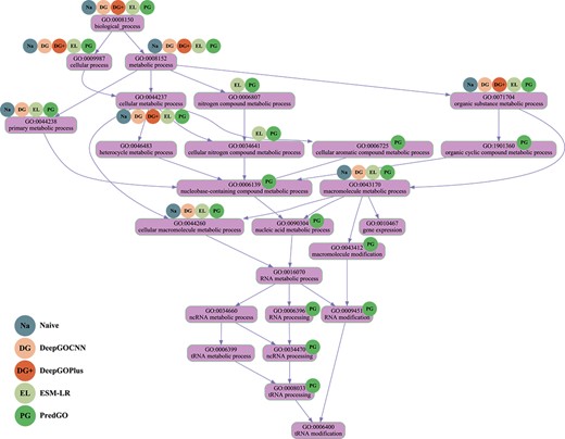
We use protein Q47319 as an example to illustrate the difference in performance between PredGO and other competing methods. Q47319 is a tRNA-uridine aminocarboxypropyltransferase that catalyzes the formation of 3-(3-amino-3-carboxypropyl)uridine (acp3U) at position 47 of tRNAs, and acp3U47 confers thermal stability on tRNA [60–62]. Figure 3 shows the DAG plot of the BPO terms of this protein and the method to correctly predict the corresponding GO terms, the Table 6 shows the specific prediction results of each method as well as the F1 scores.
DAG diagram of correct predicted BPO terms of Q47319 using different methods.
Predicted GO terms (GO terms in UniGOA16 dataset) of Q47319 in BPO by PredGO and competing methods
| Method | Results | F1 scores |
|---|---|---|
| Naive | GO:0044260, GO:0008152, GO:0043170, GO:0044763, GO:0071704, GO:0044237, GO:0050794, GO:0050789, GO:0065007, GO:0044699, GO:0050896, GO:0009987, GO:0044238 | 0.378 |
| DiamondBLAST | – | 0.000 |
| DiamondScore | – | 0.000 |
| DeepGOCNN | GO:0050794*, GO:0044699, GO:0044763, GO:0050789,GO:0043170, GO:0050896, GO:0065007, GO:0044267, GO:0071704, GO:0044238, GO:0019222*, GO:0008152, GO:0009987, GO:0019538*, GO:0044237, GO:0044260 | 0.350 |
| DeepGOPlus | GO:0044699, GO:0050789, GO:0065007, GO:0071704,GO:0008152, GO:0009987, GO:0044237 | 0.258 |
| LR-ESM | GO:0008152, GO:0044763, GO:0044699, GO:0044710*,GO:0044237, GO:0009987, GO:0034641*, GO:0006807*, GO:0043170, GO:0044238, GO:0044260, GO:0071704 | 0.5 |
| PredGO | GO:0043412*, GO:0046483*, GO:0044699, GO:0009451*,GO:0044238, | 0.864 |
| GO:0008152, GO:0044260, GO:0006396*,GO:0034470*, GO:0034641*, | ||
| GO:0071704, GO:0006139*, GO:0006725*, GO:0090304*, GO:1901360*, | ||
| GO:0043170,GO:0044237, GO:0006807*,GO:0009987, GO:0008033* | ||
| Experimental annotation | GO:0043412*, GO:0046483*, GO:0009451*, GO:0044238, GO:0008152, GO:0044260, | |
| GO:0006396*, GO:0034470*, GO:0034641*, GO:0071704, GO:0006139*, GO:0006725*, | ||
| GO:0090304*, GO:0006399*, GO:1901360*, GO:0010467*, GO:0043170, GO:0044237, | ||
| GO:0016070*, GO:0006807*, GO:0009987, GO:0006400*, GO:0008033*, GO:0034660* |
Note: The correctly predicted GO terms are in bold. Terms that do not appear in naive are added with *.
As can be seen, the Q47319 protein has a total of 24 experimentally annotated BPO terms. 20 terms were predicted by PredGO, of which 19 terms were correct and only five terms were not predicted. Compared to other competing methods, PredGO predicted a much higher percentage of terms correctly and significantly reduced the number of incorrectly predicted terms. In addition to this, PredGO predicted more specific functions and successfully predicted that the protein has a tRNA processing function. The correct prediction results for DeepGOCNN and DeepGOPlus were essentially the same as the frequency-based naive method. The same protein language model-based method LR-ESM predicted less specific GO terms. DiamondBLAST and DiamondScore based on sequence similarity could not predict the function of Q47319 protein because no homologous protein of Q47319 protein could be found in the training set.
Ablation study
To investigate the effect of the predicted structure and PPI information on the prediction performance of PredGO, we designed an ablation study. We compared four models: using only pre-trained embedding, using pre-trained embedding and predicted structure, using pre-trained embedding and PPI information, and the model PredGO using all information. These models all use MLP to transform protein embedding into GO terms embedding. The difference lies in that they either omit the structure feature extraction module, or the PPI feature fusion module, or both. The performance of these models is shown in Table 7.
Performance comparison of different feature combinations
| Features | |$\boldsymbol{F_{max}}$| | |$\boldsymbol{S_{min}}$| | AUPR | ||||||
|---|---|---|---|---|---|---|---|---|---|
| MFO | BPO | CCO | MFO | BPO | CCO | MFO | BPO | CCO | |
| pre-trained embedding | 0.651 | 0.379 | 0.679 | 4.123 | 18.708 | 5.609 | 0.559 | 0.276 | 0.706 |
| pre-trained embedding && predicted structure | 0.672 | 0.381 | 0.686 | 3.879 | 18.515 | 5.573 | 0.596 | 0.278 | 0.722 |
| pre-trained embedding && PPI | 0.667 | 0.400 | 0.683 | 4.018 | 18.217 | 5.665 | 0.576 | 0.307 | 0.710 |
| pre-trained embedding && predicted structure && PPI | 0.687 | 0.405 | 0.694 | 3.719 | 17.947 | 5.442 | 0.603 | 0.312 | 0.734 |
Note: Best performance in bold.
As can be seen from the table, the model using pre-trained embedding and predicted structure has more significant improvements in MFO and CCO compared to the model using only pre-trained embedding, with a maximum improvement of about 6.6% in metrics, and insignificant improvements in performance in BPO. Compared to the model using only pre-trained embeddings, the model using pre-trained embeddings and PPI information showed more significant improvements in BPO, with gains of over 11% in AUPR, but much smaller improvements in CCO. The model combining the pre-trained embedding, predicted structure, and PPI information has a more comprehensive prediction performance, outperforming the other three models in terms of MFO, PPO and CCO. This is because molecular function and cellular component are more related to protein structure, while biological processes are mostly generated by multiple protein interactions, which are more associated with PPI. The protein interaction information contained in the predicted structure is very limited, which leads to almost no improvement in BP performance by adding predicted structure. Therefore, we have incorporated PPI information to compensate for this.
Large-scale function prediction
We applied PredGO to predict GO functions of all 205 788 human sequences in UniprotKB. We used only sequence and PPI information for those proteins whose structures could not be predicted by AlphaFold. We extracted these proteins’ experimental and non-experimental annotations from the GOA database by referring to the CAFA rules and compared them with the prediction results of PredGO. As shown in Figure 4A, only 12.21% of protein sequences have experimental annotations in the GOA database, and 62.40% of the sequences have non-experimental annotations. As for PredGO, |$\sim $|100% entries are annotated with a confidence score greater than 0.5 (PredGO_All), and |$\sim $|90% of which are based on predicted structure (PredGO_Structure). This shows that PredGO can achieve extremely high coverage.
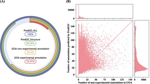
Protein function prediction results for human. (A) The percentage of human proteins in UniprotKB with annotated functions. (B) The number of functions per protein predicted by PredGO (y-axis) compared to the number of electronic annotations per protein in GOA (x-axis).
In addition, we visualized the number of annotations for each protein. Figure 4B compares the number of non-experimental annotations in the GOA database with the number predicted by PredGO. As seen from the figure, PredGO can predict more GO terms for most proteins, which means that PredGO can explore more functions.
WEB SERVER
We built a flexible and interactive web server that provides prediction and browsing services. Users can submit protein sequences or structures to the PredGO web server for function prediction (Figure 5A). The prediction results are presented in a table by default and can be downloaded as a text file (Figure 5B). It is also possible to browse the functions of all human proteins in UniprotKB predicted by PredGO (Figure 5C) and batch download all the annotations. In addition, users can interactively view the 3D structure of proteins and GO annotations in a tree (Figure 5D).
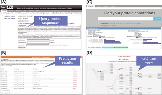
PredGO web server. (A) Enter query protein sequences; (B) prediction results; (C) database search, statistics and download; (D) visualization of GO annotations.
CONCLUSION
We designed a method called PredGO for protein function prediction, a meaningful but complex multi-label classification problem. PredGO makes full use of the massive amount of sequence information through a pre-trained protein language model, incorporates information contained in protein structure predicted with atomic precision by AlphaFold2, and fuses interacting proteins based on attention mechanisms. It is clear from the experimental results that our method enables high-performance protein function prediction. Even in the case of only sequences, high-performance prediction of MFO and CCO can be achieved without degrading the performance of BPO.
Our method faces certain challenges in predicting the funciton of long protein sequences. In the future, alternative structure prediction methods can be considered to address this issue. Furthermore, integrating more diverse and heterogeneous data sources, along with pre-training protein structure models using experimentally determined and predicted protein structures, has the potential to improve the predictive performance of the model.
We propose a protein function prediction method using heterogeneous features, including sequence, predicted protein structure and protein–protein interaction relationships, that outperforms other state-of-the-art methods in terms of coverage and accuracy.
A graph neural network combined with a geometric vector perceptron is applied to extract protein structure information.
Proteins with interactions are viewed as different words in a sentence, and sequence information and interaction information are fused by a PPI feature fusion module.
ACKNOWLEDGEMENTS
The work was carried out at National Supercomputer Center in Tianjin, and the calculations were performed on Tianhe new generation Supercomputer.
FUNDING
This work was supported by the National Natural Science Foundation of China under grants Nos 62272490 and 61972422.
AUTHORS’ CONTRIBUTION
R.Z., Z.H and L.D. conceived and designed the algorithm;, R.Z. and Z.H conducted the experiments, R.Z. analyzed the results. R.Z. and L.D. wrote and reviewed the manuscript.
DATA AVAILABILITY
The webserver and database are available at http://predgo.denglab.org/.
Author Biographies
Rongtao Zheng is a graduate student at School of Computer, Central South University, Changsha, China. His research interests include data mining and protein function prediction.
Zhijian Huang is a graduate student at School of Computer, Central South University, Changsha, China. His research interests include data mining and protein function prediction.
Lei Deng is a professor in School of Computer Science and Engineering, Central South University, Changsha, China. His research interests include data mining, bioinformatics and systems biology.
