


Abstract
Survival analysis is critical to cancer prognosis estimation. High-throughput technologies facilitate the increase in the dimension of genic features, but the number of clinical samples in cohorts is relatively small due to various reasons, including difficulties in participant recruitment and high data-generation costs. Transcriptome is one of the most abundantly available OMIC (referring to the high-throughput data, including genomic, transcriptomic, proteomic and epigenomic) data types. This study introduced a multitask graph attention network (GAT) framework DQSurv for the survival analysis task. We first used a large dataset of healthy tissue samples to pretrain the GAT-based HealthModel for the quantitative measurement of the gene regulatory relations. The multitask survival analysis framework DQSurv used the idea of transfer learning to initiate the GAT model with the pretrained HealthModel and further fine-tuned this model using two tasks i.e. the main task of survival analysis and the auxiliary task of gene expression prediction. This refined GAT was denoted as DiseaseModel. We fused the original transcriptomic features with the difference vector between the latent features encoded by the HealthModel and DiseaseModel for the final task of survival analysis. The proposed DQSurv model stably outperformed the existing models for the survival analysis of 10 benchmark cancer types and an independent dataset. The ablation study also supported the necessity of the main modules. We released the codes and the pretrained HealthModel to facilitate the feature encodings and survival analysis of transcriptome-based future studies, especially on small datasets. The model and the code are available at http://www.healthinformaticslab.org/supp/.
INTRODUCTION
Prognosis and life quality are major concerns of cancer patients but remain challenging for cancer researchers [1, 2]. Survival analysis is a routine approach to assess an event of interest by a specific time and has been improved to handle imperfect datasets with missing death dates of some censored patients [3]. Cox proportional hazard model is one of the most widely used survival analysis approaches and can handle multiple risk factors and censored samples [4, 5].
The rapid advancement of high-throughput sequencing technologies has generated an extremely high dimension of genic features, which poses a computational challenge for survival analysis. Several survival studies have chosen feature selection algorithms to reduce the feature dimensions, including L2 penalty in ridge regression [6, 7], L1 Lasso regularization [8, 9] and tree-based ensemble methods [10]. XGBLC [11] was an improved survival prediction model combining L1 regularization and ensemble learner extreme gradient boosting (XGBoost). This method was designed to avoid overfitting and to get more stable performance. However, these methods do not consider the complex intergenic correlations sufficiently and have limited ability to explore non-linear relationships.
Deep learning technologies are good at automatic extraction of complex patterns and have been used to extend the conventional Cox regression approach for the high-dimensional transcriptome-based survival analysis e.g. Cox-nnet [12]. These methods combined artificial neural networks with Cox regression models to extract the intergenic non-linear patterns within high-throughput OMIC data. Transfer learning has been widely used to avoid overfitting through the utilization of additional information from a source task. Hanczar et al. showed that transfer learning could significantly improve the cancer prediction task on a small training set of transcriptomic profiles [13]. The pretrained variational autoencoder Cox model (VAECox) [14] was another representative work, transferring genomic information from other cancer types to the survival analysis task of a specific cancer type.
A living system is highly complicated, and biological networks offer valuable information for understanding system-level patterns between genes [15–17]. Hu et al. conducted a comprehensive survey of how TFs were involved in gene expression, gene regulation and interaction, and suggested that TFs were also significantly related with cancer survival [18]. Some studies have attempted to integrate the intergene cooperative and synergistic effects in survival analysis through biological networks such as protein–protein interaction network, gene-coexpression network and gene regulatory network [19]. Zhang et al. applied the gene network information in the Cox regression approach, and the proposed Net-Cox algorithm outperformed the conventional Cox models on the prognosis prediction of ovarian cancer treatment [5]. Li et al. defined a signaling entropy calculation method to infer personalized pathway activations and quantified the dysregulations of essential pathways for survival analysis [20]. Ghosh Roy et al. used the prior signaling pathway knowledge and gene mutation information to simulate signal flow disruptions in a specific cancer type and proposed a novel Mutated Pathway Visible Neural Network architecture for the interpretable cancer survival risk prediction [21]. However, they focused on a few representative pathways, and the overall view of the gene regulatory network remained to be fully characterized.
Graph neural network is another deep learning framework to model the coexpression gene modules for the OMIC-based disease diagnosis and prognosis [22]. Graph neural networks have demonstrated powerful capabilities in extracting OMIC-based information for the classification tasks of cancer diagnosis and prognosis [23, 24]. The graph convolutional network with the embedded graph learning module (glmGCN) was designed to formulate the complex correlations of lncRNAs and mRNAs, and accurately predicted the distant metastasis of cancers [23]. A novel interpretable multi-level attention graph neural network (MLA-GNN) was proposed to formulate the intergenic coexpression patterns for disease classification and survival prediction and achieved the best performance on two cancer types and coronavirus disease 2019[22].
Research studies have shown that the gene activity patterns in normal tissues carry important information and may serve as ideal references for understanding the developmental trajectories of complex diseases such as cancer [25]. Normal control tissues are usually extracted from the adjacent regions of cancer lesions, and their close involvement in the tumor microenvironments may not accurately reflect the genic activities in the actual healthy tissues [26]. However, it is often difficult to provide the OMIC profiles of the actual healthy tissues from the same cohort of participants in clinical practice [27]. Uhlen et al. explored the associations between the gene expression levels in human solid tumors and the corresponding normal tissues and revealed that the normal tissues were more similar to the other normal samples than to the cancer samples from the same cohort of participants [28]. The complex synergetic collaboration of various regulatory factors remains to be modeled by advanced algorithms such as deep learning.
In this study, we proposed a graph attention network (GAT) framework to model the synergetic interactions of regulatory factors (HealthModel) in the gene regulatory network of healthy samples and transferred the pretrained HealthModel to the multitask survival prediction framework (DQSurv) for cancer survival analysis. The experimental procedure of this study is shown in Figure 1. Both transcription factors (TFs) and long intergenic noncoding RNAs (lincRNAs) positively contributed to the gene expression prediction based on the HealthModel-encoded latent features. We obtained a GAT-based DiseaseModel after fine-tuning the HealthModel on training cancer samples and defined the difference between the HealthModel- and DiseaseModel-encoded latent features as the dysregulation quantification of a given cancer sample. The multitask framework optimized the main task of survival analysis and the auxiliary task of gene expression prediction based on the latent features encoded by the two GAT models. The experimental data showed that DQSurv outperformed both machine learning- and deep learning-based survival analysis models on 10 popular benchmark cancer types and an independent dataset.
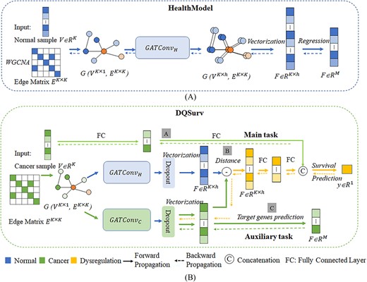
The workflow of the study. (A) The pretrained GAT architecture HealthModel and (B) the multitask survival prediction framework DQSurv, including the survival prediction task and the gene expression prediction task. The gray boxes with the letters A/B/C represent the three major modules to be described in detail in the ‘Overview of the study’ section.
The main contributions of this study include the following: (i) a multitask GAT framework was proposed to simultaneously integrate the intergenic information of both healthy and cancerous samples; (ii) the HealthModel was trained using the healthy samples and served as the reference gene regulatory network; (iii) the difference between the GAT-modeled gene regulatory networks of a cancer sample and the HealthModel could represent the dysregulatory distance of this cancer sample. The pretrained model and the source codes were released to facilitate similar studies by other researchers.
This study started with this Introduction section. The next section, ‘Materials and methods’, described the details of the datasets, the proposed framework and experimental settings. Then, all the experimental results are given and discussed in the ‘Results and discussion’ section. The concluding remarks and the limitations of this study are summarized in the ‘Conclusion’ section. The pretrained models, the code and the supplementary data are given in the sections ‘Data availability’ and ‘Supplementary data’, respectively. The other information required by the journal is given in the respective sections.
MATERIALS AND METHODS
Dataset and preprocessing
The RNA-sequencing (RNA-seq) gene expression data were downloaded from the UCSC Xena platform [29], which reanalyzed the RNA-seq raw data from The Cancer Genome Atlas (TCGA) [30] and the Genotype-Tissue Expression (GTEx) programs [31]. The reanalysis pipeline realigned the RNA-seq reads to the human genome version hg38 and recalculated the gene expression levels using RSEM [32] and Kallisto [33]. This reanalysis aimed to eliminate the batch effects of different computational processing procedures to the maximal extent and to compare the normal and cancer samples directly. Table 1 summarizes the datasets used in this study.
Healthy samples were retrieved from the GTEx dataset [31] in the UCSC Xena platform. A tissue with fewer than 10 samples was removed. A total of 7373 healthy samples from 47 tissues were collected (Supplementary Table S1). Features with >15% missing values in the healthy samples were removed, as similar in another pan-cancer analysis study [14]. A K-nearest neighbor imputation was used to fill in the remaining missing values. Z-Normalization was also done for each feature.
Cancer samples were retrieved from TCGA [30] dataset in the UCSC Xena platform. This study compared the proposed framework with two studies i.e. Cox-nnet [12] and VAECox [14]. Thus, we used the same 10 cancer types as in these two studies (Table 1). The cancer samples were labeled as ‘Censored’ and ‘Dead’ based on the annotation ‘OS’, and these numbers are summarized in Table 1. The same preprocessing strategy was used for each cancer type.
There were 16 074 transcriptomic features overlapping between the 11 datasets. The expression levels of many genes did not have large variations. Such genes would not have positive discriminative power and would significantly increase the computational requirement of training the artificial intelligence models. Therefore, 8000 features with the largest variances were kept for further analysis.
Summary of the datasets used in this study
| ID | Dataset | # Censored | # Dead | # All |
|---|---|---|---|---|
| 1 | Training | – | – | 7373 |
| 2 | BLCA | 237 | 188 | 425 |
| 3 | BRCA | 1012 | 198 | 1210 |
| 4 | HNSC | 310 | 253 | 563 |
| 5 | KIRC | 403 | 200 | 603 |
| 6 | LGG | 391 | 130 | 521 |
| 7 | LIHC | 258 | 162 | 420 |
| 8 | LUAD | 356 | 209 | 565 |
| 9 | LUSC | 300 | 242 | 542 |
| 10 | OV | 264 | 160 | 424 |
| 11 | STAD | 276 | 167 | 443 |
The first column lists the ‘Training’ dataset and the datasets of 10 cancer types. The last column ‘# All’ is the total number of samples in each dataset.
Regulatory factors
We predicted the expression levels of messenger RNAs (mRNAs) by integrating two types of regulatory factors, TFs and lincRNAs. TFs have widely been used as the regulatory factors in constructing gene regulatory networks [34, 35].
Recent studies have suggested that long noncoding RNAs (lncRNAs) are also actively involved in gene regulations and are increasingly being recognized as important regulatory factors of disease pathogenesis [36]. Zhang et al. showed that the antisense lncRNA FOXC2-AS1 upregulated FOXC2 and induced doxorubicin resistance in osteosarcoma [37]. Li et al. characterized the lncRNAs’ regulations of the immune system across multiple cancer types, showing that they could serve as potential oncogenic biomarkers [38]. lncRNAs in the intergenic regions (lincRNAs) have shown their regulatory contribution to the in vivo stress responses of de-differentiation and cell cycle [39]. Considering the difficulty in separating the RNA-seq reads of the overlapping mRNAs and lncRNAs, this study focused on the lincRNAs.
We separated the transcriptomic features into three groups, namely, TF, lincRNA and mRNA. The TF features were defined by the annotations of the Human Protein Atlas [40, 41]. The GTEx dataset provided the annotations of lincRNAs. We curated the genes in the third-level pathways in the KEGG database [42]. An mRNA feature was relocated to the TF class if it has a regulatory role for a target gene in the TRRUST database [43]. Supplementary Table S2 summarizes the KEGG pathways with >50 TFs or >100 mRNA features, which were investigated in this study. The KEGG database provides very limited information about lincRNAs. Therefore, we used all the lincRNA features as the regulatory factors of these pathways.
The final dataset had 425 TFs, 375 lincRNAs and 3062 mRNAs for the 88 KEGG pathways for further analysis.
Construction of the regulatory factor network
We formulated the complex correlations among the TFs and lincRNAs as a graph with the input features as the vectors V and an edge matrix E. A sample has K regulatory features, represented by VK × 1. There were 425 TFs and 375 lincRNAs, and the dimension of a sample was K = 425 + 375 = 800. WGCNA [44] was used to calculate the edge matrix E. The pairwise weight between two nodes vi and vj was calculated as the Pearson correlation coefficient. A gene regulatory network has some hub genes with essential roles and demonstrates the scale-free topology [45]. We used the topological overlap measure (TOM) to calculate the correlation between two features or nodes vi and vj as follows:
where the soft threshold β is calculated using the ‘pickSoftThreshold’ function in the WGCNA package; aij is the power exponential function; u is a gene, excluding i and j; and |$k=\sum_u{a}_{iu}$| is the node connectivity. WGCNA clustered the expression profiles of the transcriptomic features into multiple modules based on the commonly used dissimilarity measure (1 − TOM ≥ 0.15) as in a previous study [46].
The constructed network G(VK × 1, EK × K) was fed into the GAT layer, which is an advanced graph convolutional layer [47]. The GAT layer encodes a node as the weighted combination of its neighboring nodes and the node itself. The attention coefficient between the two nodes vi and vj was calculated as follows:
where W is the trainable weight parameter of a fully connected layer, || denotes the concatenation operation and LeakyReLU is the activation function used in this network.
Overview of the study
Figure 1A shows that the GAT-based network of regulatory factors was pretrained on the healthy samples from the GTEx dataset. This was denoted as HealthModel, which had 800 regulatory features as its input vector and predicted the expression levels of 3062 mRNA features. The mean square error (MSE) was used as the loss function for the pretraining process. The HealthModel represented the quantitative relationships between the two types of regulatory factors (TFs and lincRNAs) to mRNAs.
The multitask framework DQSurv is shown in Figure 1B. DQSurv included a feature extraction module for the regulatory factors (A), a feature extraction module for the distance quantitative description (B) and an auxiliary gene expression prediction module (C). The weights of the HealthModel were used to initialize the DQSurv’s GAT layer. Module B learned the regulatory representation difference between the control health (HealthModel) and the cancer status (DiseaseModel). The auxiliary task (module C) optimized the mRNAs’ expression predictions through the GAT-encoded latent features. The main task of DQSurv was to measure the dysregulation quantification between the HealthModel and DiseaseModel for the survival analysis task.
Details of the HealthModel
The HealthModel used 800 regulatory features and predicted the expression levels of 3062 mRNA features based on the node-encoded latent features. Let the graph network of the HealthModel be G(VK × 1, EK × K). The GAT network had K = 800 regulatory features as the nodes and each node had an expression level in the query sample S. The complex associations among these nodes were diffused across the network. Each node had eight hidden variables. Therefore, the sample S was encoded by 6400 latent features (8 hidden variables × 800 nodes). A fully connected layer was used for the regression model of the 3062 mRNA features’ expression levels, instead of the pooling layer in the traditional graph classification task [48]. The dropout rate of 0.3 was used for both the GAT and the fully connected layers. The Adam optimizer was used to optimize the GAT network, and the learning rate was set at 1e−5. The MSE was used as the loss function for the regression task. |$\hat{y}$| denotes the predicted expression levels of the 3062 mRNA features.
Multitask survival prediction model DQSurv
The DQSurv model used the node-encoding features of the GAT network to optimize the two tasks. The pretrained HealthModel extracted the regulatory representations across healthy tissues and was fine-tuned by the two tasks of DQSurv on training cancer samples (denoted as DiseaseModel). The difference between the latent features encoded by the models HealthModel and DiseaseModel was used to represent the overall regulatory change of a given sample S relative to the reference network:
where HealthModel(S) and DiseaseModel(S) are the latent features of S encoded by the HealthModel and DiseaseModel, respectively.
The main task of survival prediction integrates RegChange(S) and S as its input and outputs the log hazard ratio for cancer patients. We balanced the two tasks using the Loss-Balanced Task Weighting strategy [49], which balances the influence of the task-specific weights by considering the loss ratio between the current loss and the initial loss. We evaluated the hyperparameter loss ratio α at 0.1 and 0.5, as described in Liu et al. [49]. Supplementary Figure S1 shows that a better performance was achieved by setting the loss ratio at 0.5, which was used as the default value of this hyperparameter in the following experiments.
Loss functions
HealthModel is a GAT-based regression model to predict the expression levels of target genes. The loss function of the pretrained HealthModel used the mean square error loss (MSELoss) [50].
The loss function of the DQSurv model consisted of three parts i.e. the objective function of the Cox-PH model, the Mean Square Error loss function of the auxiliary regression task and the regularization term.
The first component of the loss function was based on the Cox-PH model, which predicts a patient’s hazard ratio [51]. The model was defined as follows:
where X is the gene expression profile of n patients and p genes, |${x}_i=\left({x}_{i1},\dots, {x}_{ip}\right)$|; θ is the log hazard ratio for patient i; and β is the trainable parameter of the model. The objective function of the Cox-PH model was a negative partial log-likelihood defined as follows:
where t is the observed or censored survival time for the |${i}^{\mathrm{th}}$| patient. The condition |${t}_j\ge{t}_i$| is used to select the patients whose survival times are longer than that of the |${i}^{\mathrm{th}}$| patient. C(i) is the indicator of whether the death event of the |${i}^{\mathrm{th}}$| patient is observed. This study defined the log hazard ratio as follows:
where W is the weight coefficient matrix between the input layer and the hidden layer, and b is the bias term of each hidden layer node.
The second component of the overall loss function was the MSE loss [Equation (9)] for the auxiliary task. The third component was the regularization term. Therefore, the overall loss was defined as shown in Equation (10).
Experimental settings
The GAT-based HealthModel was trained on 7373 healthy tissue samples from the GTEx dataset. This dataset was randomly divided into the training, validating and testing subsets at the ratio of 8:1:1. The hyperparameters were evaluated using the Bayesian optimization parameter adjustment of the PyTorch ax package on the training set. The details of the computational settings and the value ranges of parameters are listed in the Supplementary Table S3. Dropout and early stopping strategies were used to avoid overfitting. The training of HealthModel takes around 30 min and 38 GB GPU memory.
To conduct a fair comparison of the survival analysis problem, we evaluated our framework on the same 10 cancer types as the two previous studies, Cox-nnet [12] and VAECox [14]. The 10 datasets were also randomly divided into the training, validating and testing subsets at the ratio of 8:1:1. The final performance results were obtained on the testing sets. Ten random runs of the entire process on each cancer type were conducted to avoid sample selection bias.
All experiments were implemented using the PyTorch version 1.12.0 framework.
Performance evaluation metrics
The survival prediction model was evaluated using the commonly used metric, the concordance index (C-index) [52]. A larger C-index value suggests a better model. C-Index quantifies the model’s ability to correctly provide a reliable ranking of the survival time based on the individual risk scores:
where k denotes the set of validly orderable pairs when |${t}_i<{t}_j$|, and |k| represents the number of comparable pairs among them. I is the indicator function of whether the condition in parentheses is satisfied or not. P(x) is the predicted score from the model.
The overall performance on the 10 datasets was measured by the micro-average of the 10 C-index values, which takes into account the different numbers of samples in the 10 datasets [14]. The performance of the regression task across the 10 datasets can also be evaluated by the micro-average of the MSE values as follows:
where |${n}_i$| is the number of samples, |${c}_i$| is the C-index of the ith cancer type and |${m}_i$| is the MSE value of the ith cancer type.
RESULTS AND DISCUSSION
Contributions of lincRNAs and TFs to gene expression prediction
Many lincRNAs have shown their functional involvement in the gene regulatory networks [36–38], but they are rarely used in the investigations of the gene regulatory networks or gene expression predictions. We evaluated the lincRNA’s contributions to the gene expression prediction task (Figure 2). Through the comparative experiment, we measured how much improvement the regression model for the gene expression prediction task could obtain by including lincRNAs in the list of regulatory factors.
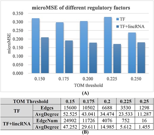
Evaluation of lincRNAs as the regulatory factors for the GAT-based gene expression prediction task. Two settings of regulatory factors were evaluated, namely, TF and TF + lincRNA. (A) The microMSE values (vertical axis) of the GAT models using TF or TF + lincRNA as the regulatory factors. Five values (0.150, 0.175, 0.200, 0.225 and 0.250) were evaluated as the TOM thresholds (horizontal axis). (B) The numbers of edges (Edges) and the average degrees of the constructed GAT graph using different TOM thresholds. The nodes with no edges were excluded from the calculation of the average degrees.
The expression prediction task of the mRNA features achieved the microMSE values between 0.200 and 0.350 using only TF features as the regulatory factors (Figure 2A). If we also included lincRNAs as the regulatory factors, the prediction models under all five TOM threshold values improved. The largest improvement (48.1%) was achieved at the TOM threshold of 0.225, and the overall smallest microMSE (0.171) was achieved at the same TOM threshold value.
Figure 2B shows a consistent trend of more edges under a smaller TOM threshold value. The GAT network consisted of 752 edges and 5.612 average degrees when it achieved the smallest microMSE (0.171). This setting was used in the following sections.
Evaluation of DQSurv for gene expression prediction
Gene expression prediction is crucial for disease-related gene regulation detection, and this part compared the gene expression prediction performance of the proposed multitask framework DQSurv with those of five regression methods, including linear regression (LR) [53], Lasso [54, 55], Multi-Layer Perceptron (MLP) [56], Neighbor Connection Neural Network (NCNN) [57] and a new long short-term memory (LSTM)-based gene expression prediction (L-GEPM) [58]. LR and Lasso are classic methods for regression. The Library of Integrated Network-based Cell-Signature program selects 1000 landmark genes to predict the remaining gene expression value using simple LR method [59]. Lasso achieves feature selection simultaneously with regression. Chen et al. used MLP to capture the non-linear regulation between the genes, which outperformed the LR model in their study [56]. Wang et al. [58] proposed a gene expression prediction model L-GEPM using the latent features learned by the LSTM neural network.
Graph neural network can be used to extract the complex hidden patterns within the gene regulatory network [60]. Li et al. proposed a novel NCNN framework to improve the gene expression prediction performance using the knowledge of adjacent genes in the gene interaction network [57]. The proposed DQSurv model was compared with this latest method NCNN. The ‘Simplified DQSurv’ version with only the GAT backbone was also evaluated to show whether the multitask framework (DQSurv) positively contributed to the gene expression prediction task.
The multitask framework DQSurv achieved the smallest microMSE (0.429) among all the evaluated methods (Figure 3). DQSurv also achieved the best MSE values on 5 of the 10 cancer datasets, and achieved the second-best MSE values on 3 datasets. Simplified DQSurv and MLP were ranked the best on two different datasets. NCNN achieved better overall performance in microMSE than L-GEPM, and even achieved the best MSE of 0.490 on the LUSC dataset. The overall regression performance of Simplified DQSurv was 0.434 in microMSE, with 0.020 smaller than that of NCNN. This might be due to that NCNN had more parameters than DQSurv and did not perform well on the small datasets in this study. The regression methods Lasso and LR performed the worst for the gene expression prediction task across the 10 datasets. The experimental data suggest that the latent features encoded by the GAT nodes of DQSurv achieve satisfying regression performance for the gene expression prediction task, and the multitask setting may further improve the regression performance.

Performance comparison of multiple regression methods for the gene expression prediction task. Each method was randomly run 10 times. The legend shows each method’s name with the average MSE value. The last group is the microMSE across the 10 cancer datasets.
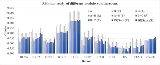
Evaluation of different module combinations. The horizontal axis lists the datasets, and the last data series ‘microC’ is the micro-average of the C-index values over the 10 datasets. The vertical axis gives the values of C-index and microC. Each dataset was randomly run 10 times. The terms R and T in the brackets represent the GAT network initialized by randomization or transferred weights from the pretrained HealthModel, respectively. Our final survival prediction model is ‘DQSurv (T)’, which is highlighted in bold.
Ablation study for the DQSurv model
As the Figure 4 shown, the final survival prediction model DQSurv was represented by ‘DQSurv (T)’ and achieved the overall best microC value (0.661). The individual modules ‘A’ and ‘B (R)’ did not rely on the transferred weights from the pretrained HealthModel, and they only achieved the microC values of 0.631 and 0.635, respectively. We further evaluated the contribution of the auxiliary task (module C) to the multitask framework. The B + C module improved the B-only network by 0.005 and 0.016 in microC under random initialization and transferred weights, respectively. This confirms the positive contribution of the auxiliary task to the survival prediction model DQSurv.
The final network used all three A/B/C modules and achieved the survival prediction performance of 0.653 (with random initialization) and 0.661 (with transfer learning) in microC. The data support the positive contributions of the three modules and the transfer learning strategy. The best module ‘DQSurv (T)’ was abbreviated as the final DQSurv model for further comparison.
Comparison with the other survival prediction studies
Our DQSurv model was compared with seven studies for the survival prediction task (Figure 5). RFCox and GBCox are the survival prediction models based on the random survival forest [10] and gradient boosted models [61]. LassoCox is the classic statistical Cox regression model with L1 regularization [62]. Cox-nnet extends the Cox regression model with an artificial neural network [12]. VAECox uses a variational autoencoder network on the RNA-seq data with the transferred weights from the pretrained model on the other cancer datasets [14]. VAECox also verifies that the survival prediction task can be improved through the transfer learning strategy. Xing et al. constructs a gene-coexpression network to explore intergene relational information and proposes a MLA-GNN for disease diagnosis and prognosis [22]. Another graph-based model glmGCN embeds the graph learning module in the graph neural network [23].
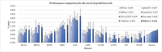
Performance comparison for the survival prediction task. The last data series ‘microC’ is the micro-average of the C-index values over the 10 datasets. Each method was randomly run 10 times. The VAECox model does not release the C-index value for each dataset, and its performance is only illustrated in the last group ‘microC.’
LassoCox outperformed the two ensemble methods, RFCox and GBCox, by 0.027 and 0.016 in microC, respectively, and the three neural network-based models achieved better survival prediction performances than the three machine learning-based Cox models i.e. LassoCox, RFCox and GBCox (Figure 5). The glmGCN model got better performance (0.607 in microC) than RFCox (0.604 in microC). MLA-GNN achieved a microC value of 0.639 and achieved the best C-index values on the LUSC and STAD datasets. MLA-GNN performed worse than Cox-nnet and VAECox in the overall performance metric microC. This might be due to that MLA-GNN only selected the top-ranked differentially expression genes to construct the network. Both VAECox and our DQSurv models used the transfer learning strategy and outperformed the Cox-nnet model by 0.001 and 0.013 in the metric microC, respectively. This suggests the positive contributions of the pretrained models on the training datasets. Both Cox-nnet and LassoCox outperformed our DQSurv model on the BRCA dataset. This might be because BRCA was the only dataset with >1000 samples, and transfer learning usually provides helpful pretrained information for small datasets [63, 64].
In summary, our DQSurv model achieved the best survival prediction performances on 5 of the 10 cancer datasets and the best overall microC value of 0.661.
Evaluation of different distance metrics
We evaluated how the survival model was affected by different quantitation ways for the dysregulation distance of the embedding features between healthy and cancer samples. The subtraction of the encoded features in the DQSurv model between healthy and normal samples was calculated as the representation of regulation changes (denoted as RegChange). We evaluated cosine distance (Cos) and Euclidean distance (EU) in replacing the subtraction method in the DQSurv model. Figure 6 shows the regression performance of different distance metrics across the datasets. The DQSurv model using Euclidean distance (DQSurv-Euc) achieved the overall performance microC of 0.648, better than that (0.633) of the DQSurv model using cosine distance (DQSurv-Cos). The DQSurv-Euc model outperformed the default DQSurv model on three datasets (BLCA, OV and STAD), while the DQSurv-Cos model achieved better performance than DQSurv on another three datasets (KIRC, LGG and LUAD). However, DQSurv achieved the best C-index values on four datasets and the best overall microC value of 0.661.
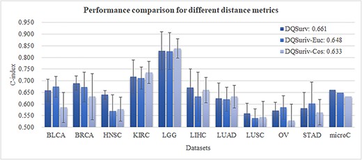
Evaluation of different distance metrics for the survival prediction task. The last data series ‘microC’ is the micro-average of the C
index values over the 10 datasets. Each method was randomly run for 10 times. The DQSurv-Euc model used Euclidean distance as the distance metric, and DQSurv-Cos used cosine distance. The default DQSurv model used the subtraction approach.
The subtraction method of DQSurv delivered a feature vector, which could be fed to the downstream prediction tasks, while Euclidean distance and cosine distance generated one distance value between two input feature vectors. Considering both the easy-to-embed subtraction feature vector and the best regression performance, we kept using the subtraction approach in the DQSurv model.
Independent evaluation of the DQSurv framework
We further evaluated our DQSurv framework on an independent dataset POG570. This cohort is a comprehensive OMIC dataset from Canada’s Michael Smith Genome Sciences Center [65]. The cohort consists of advanced and metastatic tumor patients treated in a tertiary cancer clinic, with 415 deceased and 155 living patients. The TPM-based expression levels of the RNA-seq data are available at http://bcgsc.ca/downloads/POG570/. The POG570 dataset includes 58 051 features, among which 21 253 carry missing values in fewer than 15% samples, as similar in another pan-cancer analysis study [14], and were kept for further analysis. Then, we extracted only the features corresponding to the 800 regulators and 3062 target genes, as annotated in the ‘Regulatory factors’ section. Three (ENSG00000261685, ENSG00000229729, ENSG00000250588) of the 3862 genes are absent from the POG570 dataset. Two additional genes (ENSG00000183054, ENSG00000261584) have the expression values zeros in all the samples. We padded these five genes using 0.0. The remaining data were processed by log-transformation, KNN imputation and Z-normalization. The obtained feature matrix and edge adjacency matrix were fed into the model.
Both versions of our DQSurv model outperformed the other models on the POG570 dataset (Figure 7). The detailed data of Figure 7 are given in the Supplementary Table S4. The DQSurv model with the randomized initialization (‘DQSurv (R)’) outperformed the next best model Cox-nnet by 0.001 in the metric C-index. If the pretrained HealthModel was used to initialize the DQSurv network, the ‘DQSurv (T)’ model was further improved to achieve a C-index of 0.712. The POG570 dataset has > 30 cancer types. The best survival prediction performances by both versions of DQSurv suggest the importance of capturing the cancer regulatory changes against the healthy references. We also evaluated the gene expression prediction task of DQSurv with the five regression methods, as in Table 2. DQSurv achieved the best performance with the averaged MSE of 0.439, and the Simplified DQSurv was ranked the second best with the averaged MSE 0.466.
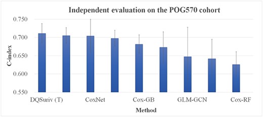
Evaluation of the survival prediction models on the independent dataset POG570. The horizontal axis gives the model names. The denotations ‘DQSurv (T)’ and ‘DQSurv (R)’ are the DQSurv models with the initial weights from the pretrained HealthModel and randomization, respectively. The vertical axis is the C-index value.
Performance comparison of multiple regression methods for the gene expression prediction task on the POG570 dataset
| Methods | Avg ± Std |
|---|---|
| Lasso | 1.013 ± 0.089 |
| LR | 0.786 ± 0.065 |
| MLP | 0.472 ± 0.056 |
| NCNN | 0.526 ± 0.042 |
| L-GEPM | 0.506 ± 0.041 |
| Simplified DQSurv | 0.466 ± 0.036 |
| DQSurv | 0.439 ± 0.039 |
| Methods | Avg ± Std |
|---|---|
| Lasso | 1.013 ± 0.089 |
| LR | 0.786 ± 0.065 |
| MLP | 0.472 ± 0.056 |
| NCNN | 0.526 ± 0.042 |
| L-GEPM | 0.506 ± 0.041 |
| Simplified DQSurv | 0.466 ± 0.036 |
| DQSurv | 0.439 ± 0.039 |
The metric MSE was used to evaluate the models, and each method was randomly run 10 times. Avg and Std refer to the average and standard deviation values of the 10 random runs of each method.
CONCLUSIONS
We introduced a GAT network to describe the complex synergetic interactions among TFs and lincRNAs in the gene regulatory network and a multitask framework DQSurv for cancer survival prediction. By fully considering the evolutionary relationship between health and cancer, we trained the HealthModel using the healthy tissues and transferred it to the fine-tuning on the training cancer samples as the DiseaseModel. This fine-tuned model learned the specific characteristics of cancers, and we defined the difference between the HealthModel- and DiseaseModel-encoded latent features as the dysregulation distance. We hypothesized that this dysregulation distance fused with the expression levels of the regulatory factors represented a more complete view of cancers. The final survival prediction model DQSurv also benefited from the auxiliary expression prediction task. The experimental data supported the contributions of the main modules and the transfer learning strategy. The pretrained models and the source codes were released to support the feature encodings and survival analysis of transcriptome-based future studies, especially on small datasets.
The main limitation of this proof-of-principle study was the dependence on high-quality transcriptomes, and substantial improvements may be needed to handle the single-cell and spatial transcriptomes with missing values. The exclusion of features with >15% missing values could also be evaluated of how the threshold (15% in this study) affects the pretrained Health model and its applications on the downstream prediction tasks.
A pretrained health model is proposed to describe the healthy gene regulation network for survival analysis.
lincRNAs are important regulatory factors in addition to TFs.
The regulations between regulators (TFs and lincRNAs) and target genes can be encoded by the graph attention model.
The distance of regulation relationships between healthy samples and cancer samples is beneficial for survival analysis.
The multitask model combines survival prediction and gene expression prediction to achieve state-of-the-art survival analysis.
ACKNOWLEDGEMENTS
The insightful comments from the four anonymous reviewers have substantially improved the convincingness and reproducibility of this study and are greatly appreciated.
FUNDING
This work was supported by the Senior and Junior Technological Innovation Team (20210509055RQ), the National Natural Science Foundation of China (62072212 and U19A2061), the Jilin Provincial Key Laboratory of Big Data Intelligent Computing (20180622002JC) and the Fundamental Research Funds for the Central Universities, JLU.
DATA AVAILABILITY
The Python implementation and the pretrained Health model and DQSurv model are freely available at http://www.healthinformaticslab.org/supp/resources.php.
Author Biographies
Meiyu Duan is a PhD student in College of Computer Science and Technology, Jilin University. Her research interests include bioinformatics algorithm design and development.
Yueying Wang is a PhD student in College of Computer Science and Technology, Jilin University. Her research interests include biomedical big data modeling.
Dong Zhao is an undergraduate student in School of Biology and Engineering, and Engineering Research Center of Medical Biotechnology, Guizhou Medical University. His research interest is about the biomedical predictions.
Hongmei Liu is a professor in School of Biology and Engineering, and Engineering Research Center of Medical Biotechnology, Guizhou Medical University. Her research interests focus on the wet and dry laboratory investigations of microbial genomics.
Gongyou Zhang is an assistant professor in School of Biology and Engineering, and Engineering Research Center of Medical Biotechnology, Guizhou Medical University. His research focuses on the bioinformatics and in vitro investigations of microbial transcription regulations.
Kewei Li is an undergraduate student in College of Computer Science and Technology, Jilin University. The research interests include bioinformatics algorithm design and development.
Haotian Zhang is an undergraduate student in College of Computer Science and Technology, Jilin University. The research interests include bioinformatics algorithm design.
Lan Huang is a professor at College of Computer Science and Technology, Jilin University, Changchun, Jilin, China. Her research interests include bioinformatics and systems biology.
Ruochi Zhang is a PhD student in School of Artificial Intelligence, Jilin University. His research interests include bioinformatics algorithm design and biomedical big data.
Fengfeng Zhou is a professor at College of Computer Science and Technology, Jilin University, Changchun, Jilin, China. His research interests include biomedical big data.
