


Abstract
Single-cell RNA sequencing (scRNA-seq) measures transcriptome-wide gene expression at single-cell resolution. Clustering analysis of scRNA-seq data enables researchers to characterize cell types and states, shedding new light on cell-to-cell heterogeneity in complex tissues. Recently, self-supervised contrastive learning has become a prominent technique for underlying feature representation learning. However, for the noisy, high-dimensional and sparse scRNA-seq data, existing methods still encounter difficulties in capturing the intrinsic patterns and structures of cells, and seldom utilize prior knowledge, resulting in clusters that mismatch with the real situation. To this end, we propose scDECL, a novel deep enhanced constraint clustering algorithm for scRNA-seq data analysis based on contrastive learning and pairwise constraints. Specifically, based on interpolated contrastive learning, a pre-training model is trained to learn the feature embedding, and then perform clustering according to the constructed enhanced pairwise constraint. In the pre-training stage, a mixup data augmentation strategy and interpolation loss is introduced to improve the diversity of the dataset and the robustness of the model. In the clustering stage, the prior information is converted into enhanced pairwise constraints to guide the clustering. To validate the performance of scDECL, we compare it with six state-of-the-art algorithms on six real scRNA-seq datasets. The experimental results demonstrate the proposed algorithm outperforms the six competing methods. In addition, the ablation studies on each module of the algorithm indicate that these modules are complementary to each other and effective in improving the performance of the proposed algorithm. Our method scDECL is implemented in Python using the Pytorch machine-learning library, and it is freely available at https://github.com/DBLABDHU/scDECL.
INTRODUCTION
As the foundational unit of various organisms, cells participate in various biological process to ensure their functions normal. The heterogeneity of cells is vital to the growth and development of complex organisms. Nowadays, single-cell RNA sequencing (scRNA-seq) permits researchers to measure gene expression levels at single-cell resolution [1]. The large amount of scRNA-seq data provides researchers with a unique opportunity to characterize different cell states and types in multicellular organisms and infer their lineage relationships [2]. Among them, the identification of cell types plays an essential role in further revealing cell heterogeneity, the complex mechanisms of cell diversity and cell function in health and diseases. However, due to the degree of noises, sparsity, batch effects and high dimensionality, it is still challenging to effectively analyze the scRNA-seq data.
To overcome this challenge, early strategies usually first reduce the dimension using various dimension reduction techniques [3], such as principal component analysis, diffusion diagram, t-Distributed Stochastic Neighbor Embedding (t-SNE) [4], Uniform Manifold Approximation and Projection [5] etc. After dimensionality reduction, traditional clustering algorithms are subsequently applied to identify different cell subgroups [6]. For example, Seurat adopts the clustering method Louvain to perform cell-community detection on the shared nearest neighbor graph [7]. CIDR introduces an implicit interpolation method to mitigate the dropout effect of scRNA-seq data, followed by classic hierarchical clustering [8]. Recently, with the development of deep neural networks, deep clustering methods have been gradually proposed for scRNA-seq data analysis. DEC utilizes an autoencoder to simultaneously learn feature representation and cluster assignments [9]. DCA adopts a zero-inflated negative binomial (ZINB) model-based loss function to characterize scRNA-seq data [10]. Similarly, scDeepCluster also adopts the ZINB model-based autoencoder to learn the latent feature embedding for the subsequent clustering [11]. scDSC is a deep structural clustering method for scRNA-seq data, which utilizes ZINB model-based autoencoder and graph neural network to integrate the structural information into deep clustering [12]. scVAE introduces a variational autoencoder to cluster scRNA-seq data [13]. ScVI approximates the underlying ZINB distribution of the observed expression values, and then performs several downstream clustering and visualization [14]. Different from the above hard clustering algorithms, scziDesk selects highly variable genes as input feature and then applies weighted soft K-means clustering to enhance the association between similar cells [15]. These deep clustering methods have made great progress in elucidating cell types of complex tissues; however, they still encounter two main difficulties.
On one hand, as the learned feature representation is critical for deep clustering methods, just using autoencoder is not enough to learn latent feature embedding from complex scRNA-seq data. Specifically, as the scRNA-seq data are obtained from different sequencing platforms, the distributions of these scRNA-seq data are not all applicable to the ZINB distribution. For example, researchers have argued that the NB distribution is sufficient for UMI-based data [16]. Differently, contrastive learning can rely on strong data augmentation to obtain robustness to dropouts. Since contrastive learning has shown great potential in feature learning [17], it is gradually utilized to learn data representation for downstream clustering. SimCLR treats different augmented versions of a given sample in a large batch as positive samples, and different augmented versions of different samples as negative samples [18]. MoCo and MoCoV2 also consider negative samples to be important for contrastive learning, and therefore explicitly maintain a queue of negative samples [19, 20]. In scRNA-seq field, to increase model robustness to the dropout event, the method contrastive-sc augments the data to expand the sample size, and adopts contrastive learning to learn the appropriate latent embedding [21], without performing explicit interpolation before clustering. Based on the contrastive learning model MOCO, Miscell also achieves the same validity without performing ZINB-based model [22].
On the other hand, the unsupervised clustering methods usually ignore the prior knowledge and neglect the distance information between similar cells. Recently, prior knowledge has been gradually available in many sequencing methods such as CITE-seq [23, 24], including both the single-cell transcriptomics data and proteomics. The usage of the prior information can contribute to more accurate and logical analysis. Recently, semi-supervised clustering can utilize a small amount of supervised information to achieve better clustering results. With prior knowledge, such as genes and protein symbols that are highly or lowly expressed in each cell type, SCINA assigns cell type identities to cells profiled by scRNA-Seq or Cytof/FACS data [25]. scDCC converts part of the prior knowledge into pairwise constraints, accordingly constructs the constraint loss and utilizes the denoising autoencoder to perform feature learning and clustering simultaneously [26]. Based on such constraints, the latent feature learning and cell type assignment can be improved. However, as these methods are based on simple pairwise constraint [27, 28], the clustering performance greatly depends on the quality of the constraint. It is usually susceptible to noisy or incorrect prior information.
Considering both merits and limitations of these previous scRNA-seq clustering methods, we propose scDECL, a novel deep enhanced constraint clustering algorithm for scRNA-seq data analysis based on contrastive learning and pairwise constraint. Specifically, based on interpolated contrastive learning, a pre-training model is trained to learn the feature embedding, and then perform clustering using enhanced pairwise constraint. In the pre-training stage, a mixup data augmentation strategy and the interpolation loss are introduced into contrastive learning to improve the diversity of the dataset and the robustness of the model. Specifically, mixup is a type of self-supervised learning in which the learner self-generates virtual instances into the training set as a combination of individual data points. In the clustering stage, for few prior label and distance information of cells, we adopt two types of transformation rules to construct enhanced pairwise constraints, and optimize the clustering with the enhanced constraints. To validate the performance of scDECL, we compare it with six state-of-the-art algorithms on different real scRNA-seq datasets. The extensive experimental results demonstrate that scDECL outperforms the competing clustering methods. In addition, we perform a detailed ablation study to evaluate the contribution of each module of scDECL in improving the model performance.
MATERIALS AND METHODS
Model framework
For exploiting the data themselves and constraint information to guide the analysis of scRNA-seq data, we propose a new deep enhanced constraint clustering algorithm based on contrastive learning, named scDECL. As shown in Figure 1, the proposed method is divided into two main stages. In the first stage, to learn effective latent feature representation of data, we conduct the contrastive learning and a pretext task learning. Specifically, to obtain a pretrained autoencoder with better parameters, the pretext task is to reconstruct the mask which is utilized to mask the scRNA-seq data. Here, we adopt a mixup data augmentation strategy. In the second stage, enhanced constraint clustering is performed on the embedded latent space. Based on two different transformation rules, the prior label and pairwise distance information of cells are into pairwise constraints, which are further merged into an enhanced pairwise constraint to optimize the clustering. In the following text, we first introduce the overall contrastive learning framework, and then elaborate data augmentation strategy, mask reconstruction and interpolation loss. Finally, we describe the construction of the enhanced pairwise constraints and the enhanced constraint clustering.
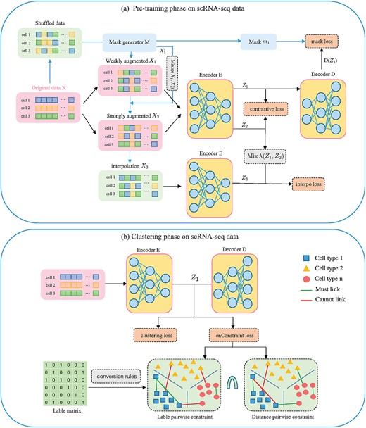
The framework of scDECL. (A) Pre-training model of scDECL. The original input |$X$| is augmented with random shuffling and generated masks |$M$| to obtain two weakly augmented versions |$X_{1}$| and |$X_{1}^{\prime }$|, and we further use the mixup data augmentation strategy to generate the strong augmented data |$X_{2}$|. Then encoder E learns the feature representation |$Z_{1}$| and |$Z_{2}$| for |$X_{1}$| and |$X_{2}$|. Both |$Z_{1}$| and |$Z_{2}$| are trained by minimizing the contrastive loss. The decoder D reconstructs the mask |$m_{1}$| from the latent embedding |$Z_{1}$|. Meanwhile, |$X_{1}$| and |$X_{2}$| are mixed up to obtain the interpolation perturbation |$X_{3}$|, which is fed into the encoder to learn the embedding |$Z_{3}$|. Then the interpolation loss is calculated based on |$Z_{3}$| and the mixup value of |$Z_{1}$| and |$Z_{2}$|. (B) Based on the learned embedding, the cells are clustered into different subpopulations, and enhanced constraints are constructed to optimize clustering, where the enhanced constraints are the intersection of label pairwise constraints and distance pairwise constraints.
Contrastive learning
Contrastive learning is a powerful approach to learn feature representations in the field of self-supervised learning. In the first stage, contrastive learning is conducted to obtain a pre-trained autoencoder and learn the effective latent feature embedding for scRNA-seq data. Here, a series of data augmentation strategies are first used to generate different inputs, and the encoder is trained to learn embedding. The contrastive loss is then computed to evaluate whether two samples are similar [26]. Contrastive loss considers the loss of positive pairs and negative pairs of samples. Specifically, given a minibatch with K samples, we define the contrastive loss as:
where |$x_{i}$| represents the sample i, and pair(i) indicates the augmented pair of sample i, |$1 \leqslant i \leqslant K$|. |$z_{i}$| and |$z_{\text{pair} (i)}$|, respectively, represents the embedding of |$x_{i}$| and pair(i). |$z_{i} \cdot z_{\text{pair} (i)}$| denotes the dot product between the normalized embedding vectors. |$\tau $| is a temperature parameter. In our experiments, the temperature parameter is set to the recommended value 0.07. The loss function intends to map similar views to adjacent representations and different views to non-adjacent representations, so that similar samples stay close to each other, while dissimilar ones are far apart in the embedded space.
As random dropout or permutation is difficult to create appropriate positive samples for data augmentation, the baseline contrastive learning still has limitations in exploiting inter-cellular information and purifying noise of data. Therefore, we improve the baseline contrastive network from three aspects. First, we utilize a mixup data augmentation strategy to strengthen the encoder training, resulting in a data-augmented version of the contrastive learning loss function. Second, we adopt the idea of interpolation to produce more samples [29], and introduce the interpolation loss function |$L_{\text{interpo }}$| in the pre-training stage, which encourages prediction of the interpolation to be consistent with the interpolation of the predictions of those points. In addition, to better explore the potential patterns and structure of the original data, our model constructs a mask matrix at the input stage, reconstructs the mask matrix based on the encoder–decoder and calculates the cross-entropy loss as the mask loss |$L_{\text{mask }}$| [30]. By masking some genes of the cells, this strategy allows the encoder to train by incomplete learning, which not only allows better exploration of the original structure but also improves the model robustness. In summary, the loss function of the current pre-training phase is calculated as
where |$L_{\text{contrast }}$|, |$L_{\text{interpo }}$| and |$L_{\text{mask }}$| represent, respectively, the contrastive loss, interpolation loss and mask loss, which are defined in the following text. And |$\mu ,\theta $| and |$ \gamma $| are the coefficients that control the relative weights of the three losses.
Data augmentation and mask estimation
In contrastive learning, data augmentation plays a significant role in model training. There are various ways to enhance the input data, such as rotation, cropping, overlay and so on [31]. However, many methods are originally proposed for image data, which are not suitable for scRNA-seq data. Recently, random dropout or alignment are widely used for the scRNA-seq data [21]. Here, in order to improve the pre-training of contrastive learning, we introduce a new strategy of data augmentation, using mixup perturbation and weak augmentation to form strong augmentation. Here, the weak augmentation refers to standard random shuffle and random mask, which masks an random set of genes in each view.
Assuming that the preprocessed scRNA-seq data of the model are |$X \in \mathbb{R}^{N \times D}$|, where N is the number of cells and D is the number of genes, each row |$x_{i}$| represents the gene expression level of the i-th cell. Specifically, to understand the intrinsic feature relationships of the data, we use a mask generator M to randomly generate a binary mask vector m:
where |$m_{i}$| is obtained by sampling from a Bernoulli distribution with probability p, and p is set as 0.7.
Then, using the mask m, the gene expression data |$x_{i}$| are mask-enhanced. That is, we utilize random mask to obtain a weak augmentation of X. The process is formalized as
where |$\bar{x}_{i}$| is a feature vector generated by randomly shuffling the features of |$x_{i}$|. We use the mask generator to generate two sets of masks |$m_{1}$| and |$m_{2}$|, then augment the data X by these two masks to obtain two augmented versions |$X_{1}$| and |$X_{1}^{\prime }$|.
where |$X_{1}$| and |$X_{1}^{\prime }$| are both generated by randomly masking X.
According to the mixup data augmentation strategy, the learner combines pairs of training instances to produce a virtual third instance. Further, we generate a weighted combination of |$X_{1}$| and |$X_{1}^{\prime }$| as the strong augmentation |$X_{2}$|:
where |$\alpha $| is the mixup parameter. For the pre-training task, |$X_{1}$| is input to the encoder. Then, the learned embedding |$Z_{1}$| is further input into the decoder to obtain the output D(|$Z_{1}$|), and the decoder reconstructs the mask |$m_{1}$| from the latent embedding |$Z_{1}$|. The mask reconstruction loss |$L_{\text{mask}}$| is calculated as the cross-entropy between |$m_{1}$| and D(|$Z_{1}$|):
Then, we can obtain a better data representation by minimizing the binary cross entropy between |$m_{1}$| and D(|$Z_{1}$|).
Interpolation-based contrastive learning
Previous research has shown that the low-density separation hypothesis is more conducive to semi-supervised learning, which inspires recent consistency-regularization semi-supervised learning methods, such as the VAT [32] and Interpolation Consistency Training. Specifically, as consistency-based regularization regulates semi-supervised learning by consistently predicting interpolation of unlabeled points, interpolation is a better choice than random perturbation [29]. Therefore, we adopt interpolation perturbation to generate more cells in the pre-training phase and make the pretrained model more robust. Figure 2 illustrates the idea of generating interpolation perturbation data.
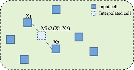
Mixing up |$X_{1}$| and |$X_{2}$| to obtain a new interpolation cell data.
Input |$X_{1}$| and |$X_{2}$| are mixed up to obtain the interpolation perturbation |$X_{3}$|, which is fed into the encoder to learn the embedding |$Z_{3}$|. After obtaining the interpolated representation, the encoder E provides predictions of the interpolation:
where |$\lambda $| is the interpolation parameter. According to extensive experiments, |$\lambda $| is set as 0.9. Based on the idea that the output of the mixup should be as close as possible to the mixup of the output, the model uses binary cross-entropy to evaluate the consistency between the interpolation |$\operatorname{Mix} \lambda (\mathrm{E}(\mathrm{X_{1}} ), \mathrm{E}(\mathrm{X_{2}} )=\operatorname{Mix} \lambda (Z_{1}, Z_{2} )$| and the model prediction |$Z_{3}=\mathrm{E}(\operatorname{Mix} \lambda (\mathrm{X_{1}}, \mathrm{X_{2}} )) $|:
Enhanced constrained clustering
For semi-supervised clustering, it is common to utilize some prior knowledge to optimize the clustering. The widely used constraint information include pairwise constraints (must-link and cannot-link) and label constraints (positive and negative labels) [33–35]. For example, the method scDCC utilizes pairwise constraints to adjust the clustering. The performance of clustering methods depends on the quality of the constraints [27]; however, single constraint is susceptible to noisy or incorrect constraints. To solve this issue, we construct enhanced constraints to optimize the clustering.
Converting label constraints. First, we construct pairwise constraint matrices through transforming the given label constraints. Assuming that the prior label information is an |$n*d$| data matrix LM, where each row |$lm_{i}$| indicates the i-th cell belonging to a certain cluster. For each row, only one element is 1, others are -1, representing that this cell belongs to the corresponding cluster. The pairwise constraint is an |$n*n$| matrix |$M^{G}=\left [M^{G}_{(i j)}\right ]$|, which is different from label constraints. Therefore, to effectively utilize these two type of constraints, we need to convert them into a uniform representation. For the label constraint, to represent and preserve prior information constraints among cells, we convert LM to a pairwise matrix |$M^{G}$| based on the following rules:
Assuming that |$L_{i}$| and |$L_{j}$| are the labels of cell |$c_{i}$| and cell |$c_{j}$|, if |$L_{i}$| and |$L_{j}$| are the same positive label, there is a must-link constraint between |$c_{i}$| and |$c_{j}$|. If |$L_{i}$| and |$L_{j}$| are different positive labels, they should have a cannot-link constraint. The pairwise matrix |$M^{G}$| can be defined as
According to the above rules, the pairwise constraint matrix |$M^{G}$| is converted from the label matrix LM, which can be further used to optimize the clustering phase.
Obtaining enhanced pairwise constraints. The CITE-seq PBMC dataset contains the read counts of messenger RNAs and proteins. Based on the normalized protein read counts, we can further calculate the Euclidean distances for all cell pairs, which can be regarded as the pairwise distance constraints among cells. Then, we utilize the distance constraint information to construct an |$n*n$| pairwise constraint matrix |$M^{D}$|. As in previous method scDCC, cells pairs with pairwise distances less than the 0.5th percentile of all pairwise distances is assigned a positive label, whereas those cell pairs with pairwise distances greater than the 95th percentile is a negative label. Finally, the two constructed pairwise constraints matrices |$M^{G}$| and |$M^{D}$| are integrated to enhance pairwise constraint matrix |$M^{R}$|. The process is formalized as
As illustrated in Figure 3, the green square with ‘+’ will be stored in the |$M^{R}$| matrix only when the labels at two identical positions in the matrices |$M^{G}$| and |$M^{D}$| are positive. On the contrary, only if the same positions in both matrices are orange, it will set as orange in the matrix |$M^{R}$|. If the relationship between |$c_{i}$| and |$c_{j}$| in |$M^{G}$| and |$M^{D}$| are different, indicating that constraint information is controversial, then, in the enhanced constraint matrix, there is not a constraint between |$c_{i}$| and |$c_{j}$|, which represents as a blue square in |$M^{R}$|.
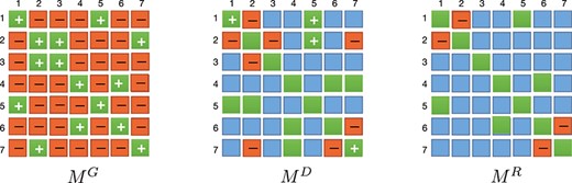
Integrating pairwise constraint matrix |$M^{G}$| and |$M^{D}$| into enhanced constraint matrix |$M^{R}$| with higher quality. The green square with ‘+’ in |$M^{G}$| and |$M^{D}$| indicates, respectively, |$M^{G}_{(i j)}=1$| and |$M^{D}_{(i j)}=1$|. The orange square with ‘-’ indicates, respectively, |$M^{G}_{(i j)}=-1$| and |$M^{D}_{(i j)}=-1$|. The blue color means that the constraint information is not clear, and |$M^{D}_{(i j)}=0$|. Since the square in diagonal line represents the constraints with itself, it is no longer represented by the ‘+’ sign in |$M^{R}$| and is not included in the constraint set.
According to these rules, we select better quality information for the clustering constraint. It is worth noting that the final |$M^{R}$| matrix contains less information than |$M^{D}$| and |$M^{G}$|. Since we randomly select 10|$\%$| of the labels to construct the label constraint matrix, the information is enough for us to subsequently build pairwise constraints.
Deep enhanced constrained clustering. Based on learned embedded latent vector |$Z_{1}$|, scDECL performs K-means clustering. Here, we define the clustering loss function as the Kullback–Leibler (KL) divergence between P and Q:
where |$q_{ij}$| is the soft label of embedded point |$z_{i}$|. Specifically, |$q_{ij}$| measures the similarity between point |$z_{i}$| and cluster center |$\mu _{j}$| calculated by the Student t-distribution [36]. |$p_{ij}$| represents the target distribution, which is derived from |$q_{i j}$|. At each iteration, minimizing the loss function |$L_{cluster}$| will make Q moving toward the derived target distribution P.
Based on the resulted clusters, we utilize the enhanced pairwise constraints matrix |$M^{R}$| to fine-tune the clustering process. From this matrix, enhanced cannot-link (CL) and must-link (ML) pairwise constraints are respectively chosen, where the must-link constraint encourages the related two cells to have the same soft label.
In contrast, two cells with cannot-link are required to have different soft labels.
where |$q_{ij}$| is the soft label of embedded point |$z_{i}$|, |$q_{aj}$| and |$q_{bj}$| is chosen in the matrix |$M^{R}$|, The enhanced constraint loss consists of the above two losses:
Therefore, the loss function of the clustering stage is defined as
|$L_{\text{cluster}}$| is presented by Equation 15. In summary, the loss function of the model is calculated as
Datasets
To evaluate the performance of the proposed algorithm, we conduct the experiments on six real scRNA-seq datasets to compare it with six state-of-the-art clustering algorithms. These scRNA-seq datasets contain label information as a prior, which is validated in previous studies. The detailed characteristics of these datasets are summarized in Table 1.
Summary Of the real scRNA-seq datasets
| Datasets | Sequencing platform | Cells | Genes | Subtypes |
|---|---|---|---|---|
| Mouse bladder cells | Microwell-seq | 2746 | 20 670 | 16 |
| Worm neuron cells | sci-RNA-seq | 4186 | 13 488 | 10 |
| 10X PBMC | 10X | 4271 | 16 449 | 8 |
| Human kidney cells | 10X | 5685 | 25 215 | 11 |
| CITE-seq PBMC | CITE-seq | 8617 | 4293 | 12 |
| Macosko mouse retina cells | Drop-seq | 14 653 | 11 422 | 39 |
For these scRNA-seq datasets obtained from different platforms, we perform data pre-processing based on their characteristics. We first filter out genes that are not expressed in any cell that does not capture any reads. Then, we normalize the data and transform the data by logTPM. In addition, we select the first 2000 genes with high variance for training, which can improve training efficiency and save training costs.
Evaluation metrics
To effectively validate the proposed method, three widely used metrics are utilized to evaluate the clustering performance, including clustering accuracy (ACC), normalized Mutual Information (NMI) and adjusted Rand Index (ARI). The larger value means higher concordance between the predicted labels and the real labels.
Clustering accuracy (ACC) can be defined as the match between the predicted clustering assignment and the true clusters. ACC is calculated as
where |$\delta (x_{1},x_{2})$| is an indicator function, if |$x_{1}=x_{2}$| then |$\delta (x_{1},x_{2})=1$|, otherwise |$\delta (x_{1},x_{2})=0$|.
NMI is used to measure the similarity between two clustering results and is a normalized form of mutual information. NMI is defined as
where |$MI=\sum _{i=1}^{N}\sum _{j=1}^{C}p_{i,j}log\left ( \frac{p_{i,j}}{p_{i},p_{j}} \right )$| calculates the mutual information between |$Y$| and |$U$|, |$H(Y)=-\sum _{i=1}^{N}p_{i}log(p_{i})$| and |$H(U)=-\sum _{j=1}^{C}p_{j}log(p_{j})$|, respectively, represent the information entropy of label vectors |$Y$| and |$U$|. |$F(x_{1},x_{2})$| can be |$max$|, |$min$| or |$mean$| function, here we choose the |$max$| function.
The ARI is adjusted based on the Rand Index (RI), which measures the consistency of the predicted clustering assignment with the true clusters. By calculation, we assume that the overlap between the two label groups |$Y$| and |$U$| is summarized in the contingency table |$R$|. Each item in table |$R$| represents the number of objects shared between |$Y$| and |$U$|; then ARI can be defined as
where (.) denotes the binomial coefficient, |$n_{ij}$| denotes the data in the contingency table |$Y$|, |$a_{i}$| is the sum of the |$i$| line of |$Y$| and |$b_{j}$| is the sum of the |$j$| column of |$Y$|.
RESULTS
Model and Hyper-parameter
We implement our model based on an autoencoder, which consists of several stacked linear layers. Specifically, the size of the autoencoder is (256, 64, 32, 64, 256), and the size of the embedding layer is 32. And each layer is followed by a ReLU activation function.
For the hyperparameters, we conduct extensive experiments to determine their optimal values. Specifically, the |$\mu $|, |$\theta $| and |$\gamma $| is set to 1, 2, 1. In Equation 7, |$\alpha $| ranges from 0.8 to 0.95. For the corresponding six datasets in Table 1, the recommended values, respectively, are 0.85, 0.9, 0.8, 0.85, 0.85, 0.95. In Equations 9 and 10, |$\lambda $| is set as 0.9, which is chosen experimentally from the range [0.5,0.9], and Figure 4 shows the impact of different parameter values on the six datasets. For the optimizer, we use Adam and Adadelta for the self-supervised pre-training stage and fine-tuning stage, respectively. The initial learning rate of the Adam optimizer is set to 0.001, and the parameters of the Adadelta optimizer are set as lr=1.0 and rho=0.95. Then we pre-trained the Autoencoder for 300 epochs. We randomly select 10|$\%$| of the total cells as the holdout cell set to generate pairwise constraints and left the remaining cells for evaluation. Specifically, we randomly select 1000, 2000, 3000, 4000 and 5000 cell pairs from the holdout cell set and construct Must-link and Cannot-link constraints based on the collected label information. We then run scDECL on the entire dataset using the generated constraints and evaluate the clustering performance on the remaining 90|$\%$| of cells.
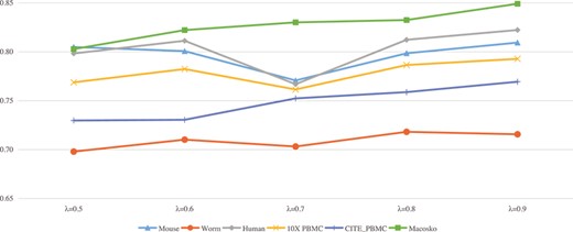
Performance comparison (NMI) of scDECL on six real datasets under different |$\lambda $| parameters.
Performance of scDECL with different number of pairwise constraints
To evaluate the effectiveness of the pairwise constraints, we compare the clustering performance of scDECL with different number of constructed pairwise constraints. Specifically, we construct 0, 1000, 2000, 3000, 4000, and 5000 pairwise constraints for four representative scRNA-seq datasets, including Human kidney cells, Worm neuron cells, Mouse bladder cells and 10X PBMC datasets. Meanwhile, scDECL is compared with the previous method scDCC, which is also based on constraint clustering.
Figure 5 shows the performance of scDECL and scDCC evaluated by ARI, NMI and ACC on these four datasets. Overall, when the number of pairwise constraints increases from 0 to 2000, we observe that the performance of scDECL achieves a significant improvement on the four datasets. And it is worth noting that when the number of pairwise constraints is above 3000, the clustering performance is not obviously better, indicating that more pairwise constraints are not simply better. Therefore, we construct 1000 pairwise constraints for the following analysis. Furthermore, compared with the competing constraint clustering method scDCC, scDECL achieves better clustering performance with different number of pairwise constraints, indicating that our constructed enhanced constraints are effective in exploiting the prior information and optimizing the clustering process.
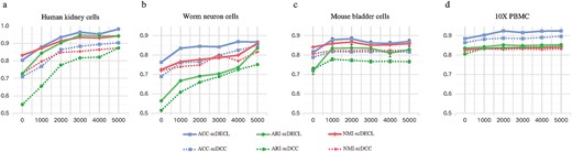
Performances comparison of scDECL and scDCC with different number of pairwise constraints on four representative datasets. The clustering performance is measured by ACC, NMI and ARI. (A) Human kidney cells. (B) Worm neuron cells. (C) Mouse bladder cells. (D) 10X PBMC cells.
Performance comparison with previous methods
To further validate the performance of scDECL, we compare it with six competing clustering algorithms on six real scRNA-seq datasets. These competing methods include scDSC [12], contrastive-sc, scDCC, scDeepCluster, Seurat and SIMLR. Specifically, scDSC is a new deep clustering algorithms based on deep graph network. contrastive-sc is a classical application of contrastive learning to scRNA-seq data analyis. scDCC is a semi-supervised method for scRNA-seq data using pairwise constraints. scDeepCluster learns feature representation and cluster based pm a ZINB distribution (ZINB) model, which simulates the distribution of scRNA-seq data. Seurat adopts the traditional clustering method Louvain to perform cell-community detection on the shared nearest neighbor graph. SIMLR combines multiple cores to learn the similarity between samples and perform spectral clustering. Here, we adopt three widely used metrics to evaluate the clustering performance of these methods, including accuracy (ACC), ARI and NMI. For the three metrics, higher scores imply better clustering performance.
Figure 6 shows the performance comparison among scDECL, contrastive-sc, scDCC, scDeepcluster, scDSC, seurat and SIMLR on the six real scRNA-seq datasets. As described in the previous section, scDECL uses 1000 pairwise constraints for the fair performance comparison. Overall, we observe that the proposed scDECL performs better and more robust than six competitive methods. For the metric ACC, scDECL achieves the best performance on all six analyzed datasets. For the metrics NMI and ARI, scDECL also outperforms the competing methods on five datasets, except the datasets 10X PBMC and worm. On the 10X PBMC datasets, scDECL is the suboptimal method, whose NMI is not as good as scDSC. According to the clustering results, we observe that the identified clusters are more structurally closed than other datasets. It might be the reason that the deep structural clustering method scDSC performs better on 10X PMBC.
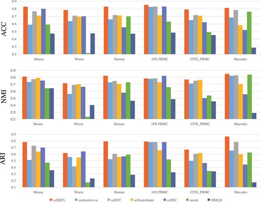
Performances comparison of scDECL, contrastive-sc, scDCC, scDeepcluster, scDSC, seurat and SIMLR, measured by ACC, NMI, ARI.
Specifically, on the Human kidney cells dataset, compared with the method contrastive sc, our proposed method significantly improves by 26.98|$\%$| on ARI, 9.47|$\%$| on NMI and 16.88|$\%$| on ACC. On the Mouse bladder cells, compared with the suboptimal method scDSC, our proposed algorithm improves by 8.32|$\%$| on ARI, 5.59|$\%$| on NMI and 2.73|$\%$| on ACC. Our method scDECL also outperforms the compared methods on the large Macosko mouse retina cells dataset. Compared with the method scDCC, our method scDECL increases by 8.13|$\%$| on ARI, 2.78|$\%$| on ACC and 2.06|$\%$| on NMI.
To intuitively validate the capability of our proposed model in learning the low-dimensional representation of high-dimensional data, we utilize t-SNE to project the feature embedding learned from the coding layer into two-dimensional space. Figure 7 shows the visualization of the identified clusters of scDECL on the six real datasets. In the figure, each point represents an cell, and each color indicates different cell type. Meanwhile, as shown in Figure 7(a) and 7(b), we compare in detail the results of scDECL and six competing methods on mouse bladder cells and worm neuron cells, which are two real datasets with more subtypes and higher complexity. Specifically, on the Worm dataset, scDECL, scDCC and scDSC can identify different types of clusters in a sparse manner, whereas the identified clusters of the other methods are dispersed, and the boundaries between clusters are mixed. Compared with the six competing methods, the proposed method scDECL achieves a good separation among different clusters.
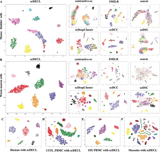
The visualization of the identified clusters of scDECL and six competitive methods. Each point represents a cell, and each color indicates different cell type. (A) The worm neuron cells. (B) The mouse bladder cells. (C) The human kidney cells. (D) The CITE-seq PBMC cells. (E) The 10X PBMC cells. (F) The macosko mouse retina cells.
Ablation study
Furthermore, we perform an ablation study to evaluate the effect of introducing the mask estimation pre-task, interpolation loss and mixup data augmentation strategy in scDECL. Therefore, we, respectively, set three variants of scDECL, including scDECL (without mask) (removing mask estimation to validate the effectiveness of mask pretask), scDECL (without interpolation) (removing interpolation to validate the effectiveness of the interpolation loss) and scDECL (without augmentation) (removing mixup augmentation to validate the effectiveness of mixup strategy). Figure 8 shows the performance comparison of scDECL and its three different variants. We observe that scDECL achieves better performance than its three variants. Specifically, the mixup data augmentation strategy improves the clustering accuracy in these representative datasets, which is especially obvious for the human kidney cells and worm neuron cells datasets. The result indicates that the three aspects all contribute in improving the performance of the proposed model.
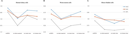
Ablation experiments on three representative datasets, comparing performance of scDECL and its three different variants with under 2000 pairwise constraints.
To validate the effect of enhanced pairwise constraints, we particularly compare the performance of scDECL with different pairwise constraint, including enhanced pairwise constraints, normal pairwise constraints and broken pairwise constraints. Figure 9 shows the performance comparison of scDECL with these three different pairwise constraints on the dataset CITE-seq PBMC. The broken pairwise constraints are pairwise constraints formed by Ed(|$c_{i},c_{j}$|) greater than 95th percentile but |$L_{i}$| is equal to |$L_{j}$|, and Ed(|$c_{i},c_{j}$|) less than 0.5th percentile but |$L_{i}$| is not equal to |$L_{j}$|. Specifically, the number of constraints ranges from 0 to 5000. As shown in Figure 5, when the number of constrains arrives 1000, scDECL can achieve good performance. As the comparison analysis also includes other clustering method without prior constraint information, we only use 1000 pairwise constraints for fair comparison. We also observe the result of enhanced pairwise constraints is significantly better than normal pairwise constraints alone. In addition, the broken pairwise constraints leads to worse performance.
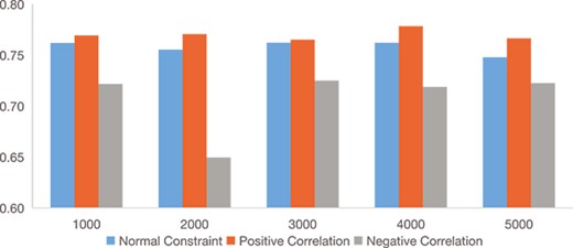
Ablation experiments on CITE-seq PBMC datasets, comparing performance (evaluated by NMI) of scDECL with normal, enhanced and broken pairwise constraints.
CONCLUSION
scRNA-seq measures transcriptome-wide gene expression at single-cell resolution, which enables researchers to characterize cell types and cell-to-cell heterogeneity in complex tissues. However, as scRNA-seq data are subject to noises, high dimensionality and dropout events, existing methods usually encounter difficulties in capturing the intrinsic patterns and structures of cells, and seldom utilize prior knowledge, resulting in clusters that mismatch with the real situation. To address these issues, we propose scDECL, a novel deep enhanced constraint clustering algorithm for scRNA-seq data analysis based on contrastive learning. Specifically, based on interpolated contrastive learning, a pre-training model is trained to learn the feature embedding, and then perform clustering based on constructed enhanced constraint. In the pre-training stage, a new data augmentation strategy and interpolation loss are introduced to improve the robustness. In the clustering stage, the prior information of the cells is converted into enhanced pairwise constraints to optimize the clustering. We compare scDECL with six competing algorithms on six real scRNA-seq datasets. The experimental results demonstrate the proposed algorithm achieves better performance. In addition, the ablation studies on each module of the algorithm indicate that these modules are complementary to each other and effective in improving the performance of the proposed algorithm.
Further, with the advent of more scRNA-seq techniques, we can obtain more information between cells, so we hope to not only rely on labeled tags to make judgments but can combine multiple aspects of information for a more comprehensive clustering effect. Therefore, since dimensionality reduction methods and labeling information will be increasingly crucial for scRNA-seq analysis, we hope this article shows the prospect of using the following principles of semi-supervised learning for scRNA-seq analysis, and it provides an example of implementation to guide future research on semi-supervised learning of genetic data.
We propose a novel deep enhanced constraint clustering algorithm scDECL for scRNA-seq data analysis based on contrastive learning. Specifically, based on interpolated contrastive learning, a pre-training model is trained to learn the feature embedding, and then perform clustering based on constructed enhanced constraint.
In the pre-training stage, a new data augmentation strategy and interpolation loss are introduced to improve the robustness. In the clustering stage, the prior information of the cells is converted into enhanced pairwise constraints to optimize the clustering.
The experimental results on six real scRNA-seq datasets show that scDECL achieves better performance compared with state-of-the-art methods.
ACKNOWLEDGEMENTS
We would like to thank MS. Huichun Zhu for fruitful discussions, and MS. Xingyu Huang for assistance in Python implementation.
FUNDING
This work were sponsored in part by the National Natural Science Foundation of China (62172088) and Shanghai Natural Science Foundation (21ZR1400400).
DATA AVAILABILITY
The datasets were derived from the following sources in the public domain: the Mouse bladder cells datasets from https://figshare.com/s/865e694ad06d5857db4b, the Worm neuron cells datasets from http://atlas.gs.washington.edu/worm-rna/docs, the 10X PBMC datasets from https://support.10xgenomics.com/single-cell-gene-expression/datasets/2.1.0/pbmc4k, the human kidney cells from https://github.com/xuebaliang/scziDesk/tree/master/dataset/Young, the Macosko mouse retina cells from https://scrnaseq-public-datasets.s3.amazonaws.com/scater-objects/macosko.rds, the CITE-seq PBMC from https://github.com/canzarlab/Specter/tree/master/data.
Author Biographies
Yanglan Gan is a professor in the School of Computer Science and Technology at Donghua University, Shanghai, China. She received the PhD degree in Computer Science from Tongji University in 2012, China. She has worked as a Visiting Scholar in the Department of Computer Science and Engineering at Washington University in St. Louis from 2009 to 2011, USA. Her research interests include bioinformatics, data mining, and Web services. She has published more than 40 papers on international journals and conferences, including Bioinformatics, IEEE/ACM TCBB, BMC Bioinformatics, BMC Genomics, Knowledge-based Systems, and Soft Computing. She served as a program committee member on BIBM 2021 and GIW 2018. She worked as a reviewer for a variety of international journals and conferences, such as BMC Bioinformatics, IEEE TCBB, Knowledge-based Systems.
Yuhan Chen is currently a master student in the School of Computer Science and technology, Donghua University, China. Before that, he received a Bachelor degree in Henan Polytechnic University, 2021. Her research interests include data mining and bioinformatics.
Guangwei Xu is a professor in the School of Computer Science and Technology at Donghua University, Shanghai, China. He received the M.S. degree from Nanjing University, Nanjing, China, in 2000, and the PhD from Tongji University, Shanghai, China, in 2003. His research interests include data secure storage, data integrity verification and privacy protection, secure computing and sharing of outsourced data, QoS and routing of the wireless and sensor networks.
Wenjing Guo is an assistant professor in the School of Computer Science and Technology at Donghua University, Shanghai, China. He received the PhD degree from East China Normal University, Shanghai, China, in 2014. His research interests include data mining, routing of the wireless and sensor networks.
Guobing Zou is an Associate Professor in the School of Computer Engineering and Science, Shanghai University, China. He received his PhD in Computer Science from Tongji University, Shanghai, China, 2012. His current research interests focus on data mining, intelligent algorithms and services computing. He has published around 70 papers on premier international journals and conferences,including Information Sciences, Expert Systems with Applications, Knowledge-Based Systems, IEEE Transactions on Services Computing, AAAI, ICWS and ICSOC.
REFERENCES
